Hospital Data Analysis Workflow Tools • healthyR

Overview

To view the full wiki, click here: Full healthyR Wiki

healthyR is a comprehensive R package designed to streamline hospital data analysis workflows. It provides a consistent, intuitive framework for analyzing common administrative and clinical data problems, helping healthcare analysts and data scientists quickly generate insights from hospital data.

Key Features

📊 Time Series Analysis: Advanced tools for analyzing hospital census, length of stay (LOS), readmission rates, and other temporal metrics
📈 Visualization: Ready-to-use plotting functions for common healthcare analytics use cases
🏥 Service Line Grouping: Automated patient classification into service lines based on ICD-10 codes and DRG
📉 Performance Metrics: Calculate and visualize key hospital performance indicators including ALOS (Average Length of Stay), readmission rates, and LOS/Readmit indices
🎨 Accessible Design: Color-blind friendly palettes and themes for inclusive data visualization
🔧 Utility Functions: Helper functions for data manipulation, Excel export, and SQL-style string operations

What Problems Does healthyR Solve?

healthyR takes the guesswork out of common hospital data analysis tasks:

Calculate average length of stay across different time periods and patient populations
Analyze readmission rates and identify trends
Create service line classifications from diagnosis and procedure codes
Generate publication-ready visualizations of hospital metrics
Perform census and capacity planning analyses
Identify outliers and excess utilization patterns

Installation

You can install the released version of healthyR from CRAN with:

install.packages("healthyR")

And the development version from GitHub with:

# install.packages("devtools")
devtools::install_github("spsanderson/healthyR")

Quick Start

library(healthyR)
library(dplyr)
library(timetk)

# Load your hospital data
# Analyze time series patterns with time signatures
data_with_time_features <- ts_signature_tbl(
  .data = your_data, 
  .date_col = admission_date
)

# Visualize average length of stay trends
ts_alos_plt(
  .data = your_data,
  .date_col = discharge_date,
  .value_col = length_of_stay,
  .by_grouping = "month"
)

# Create service line classifications
data_with_service_line <- your_data %>%
  mutate(
    service_line = service_line_vec(
      .data = .,
      .dx_col = principal_dx,
      .px_col = principal_px,
      .drg_col = drg_number
    )
  )

Core Functionality

Time Series Analysis

healthyR provides powerful tools for temporal analysis of hospital data.

Time Signature Features

Add time-based features to your data for advanced analysis:

library(healthyR)
library(timetk)

ts_signature_tbl(.data = m4_daily, .date_col = date)
#> # A tibble: 17,578 × 31
#>    id    date       value index.num  diff  year year.iso  half quarter month
#>    <fct> <date>     <dbl>     <dbl> <dbl> <int>    <int> <int>   <int> <int>
#>  1 D410  1978-06-23 9109. 267408000    NA  1978     1978     1       2     6
#>  2 D410  1978-06-24 9103. 267494400 86400  1978     1978     1       2     6
#>  3 D410  1978-06-25 9116. 267580800 86400  1978     1978     1       2     6
#>  4 D410  1978-06-26 9116. 267667200 86400  1978     1978     1       2     6
#>  5 D410  1978-06-27 9106. 267753600 86400  1978     1978     1       2     6
#>  6 D410  1978-06-28 9094. 267840000 86400  1978     1978     1       2     6
#>  7 D410  1978-06-29 9094. 267926400 86400  1978     1978     1       2     6
#>  8 D410  1978-06-30 9084. 268012800 86400  1978     1978     1       2     6
#>  9 D410  1978-07-01 9081. 268099200 86400  1978     1978     2       3     7
#> 10 D410  1978-07-02 9047. 268185600 86400  1978     1978     2       3     7
#> # ℹ 17,568 more rows
#> # ℹ 21 more variables: month.xts <int>, month.lbl <ord>, day <int>, hour <int>,
#> #   minute <int>, second <int>, hour12 <int>, am.pm <int>, wday <int>,
#> #   wday.xts <int>, wday.lbl <ord>, mday <int>, qday <int>, yday <int>,
#> #   mweek <int>, week <int>, week.iso <int>, week2 <int>, week3 <int>,
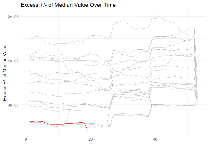
#> #   week4 <int>, mday7 <int>

Median Excess Visualization

Identify patterns and outliers in time series data:

library(healthyR)
library(timetk)
library(dplyr)

ts_signature_tbl(.data = m4_daily, .date_col = date, .pad_time = TRUE, id) %>%
    ts_median_excess_plt(
        .date_col           = date
        , .value_col        = value
        , .x_axis           = week
        , .ggplot_group_var = year
        , .years_back       = 5
    )

Visualization Tools

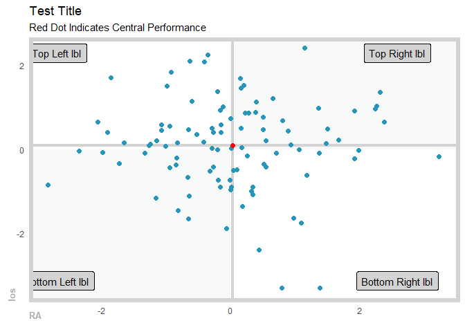
Gartner Magic Chart

Create quadrant charts for performance analysis (e.g., comparing length of stay vs readmission risk):

suppressPackageStartupMessages(library(healthyR))
suppressPackageStartupMessages(library(tibble))
suppressPackageStartupMessages(library(dplyr))

gartner_magic_chart_plt(
  .data = tibble(x = rnorm(100, 0, 1), y = rnorm(100, 0, 1))
  , .x_col = x
  , .y_col = y
  , .y_lab = "los"
  , .x_lab = "RA"
  , .plot_title = "Test Title"
  , .top_left_label = "Top Left lbl"
  , .top_right_label = "Top Right lbl"
  , .bottom_left_label = "Bottom Left lbl"
  , .bottom_right_label = "Bottom Right lbl"
)

Service Line Analysis

Automatically classify patients into service lines based on clinical codes:

# Example: Classify patients by service line
df <- data.frame(
  dx_col = "F10.10",  # ICD-10 diagnosis code
  px_col = NA,         # Procedure code (if applicable)
  drg_col = "896"      # DRG number
)

service_line_vec(
  .data = df,
  .dx_col = dx_col,
  .px_col = px_col,
  .drg_col = drg_col
)

Function Categories

📊 Time Series & Plotting Functions

ts_signature_tbl() - Add time-based features to your data
ts_alos_plt() - Plot average length of stay over time
ts_readmit_rate_plt() - Visualize readmission rates
ts_median_excess_plt() - Identify excess utilization patterns
ts_census_los_daily_tbl() - Calculate daily census and LOS metrics
ts_plt() - General time series plotting

📈 Performance Metrics

los_ra_index_summary_tbl() - Calculate LOS and readmission indices
los_ra_index_plt() - Visualize performance indices
gartner_magic_chart_plt() - Create quadrant performance charts
diverging_bar_plt() - Show positive/negative deviations
diverging_lollipop_plt() - Lollipop charts for variance analysis

🏥 Data Transformation Functions

service_line_vec() - Classify patients into service lines
service_line_augment() - Add service line column to your data
category_counts_tbl() - Get frequency counts by category
top_n_tbl() - Extract top N records by criteria
named_item_list() - Create named lists for Excel export

🎨 Accessibility Features

color_blind() - Color-blind friendly palette
hr_scale_fill_colorblind() - ggplot2 fill scale for accessibility
hr_scale_color_colorblind() - ggplot2 color scale for accessibility

🔧 Utility Functions

save_to_excel() - Export data to Excel with timestamp
opt_bin() - Calculate optimal bin size for histograms
sql_left(), sql_right(), sql_mid() - SQL-style string operations

Documentation

📚 Function Reference - Complete documentation of all functions
🚀 Getting Started Vignette - Detailed introduction and tutorials
📰 News & Changelog - Latest updates and changes

Data Included

healthyR includes reference datasets for service line classification:

dx_cc_mapping - ICD-10 diagnosis code mappings for condition categories
px_cc_mapping - ICD-10 procedure code mappings for procedure categories

Contributing

We welcome contributions! Please see our Contributing Guidelines for details on:

Reporting bugs
Suggesting new features
Submitting pull requests
Code of conduct

Getting Help

If you encounter issues or have questions:

Check the function documentation
Review the Getting Started vignette
Search existing issues
Open a new issue with a reproducible example

Citation

If you use healthyR in your research or publications, please cite it:

citation("healthyR")

License

Author

Steven P. Sanderson II, MPH - Website: https://www.spsanderson.com - GitHub: @spsanderson - ORCID: 0009-0006-7661-8247