Getting Started with healthyR.ai

First of all, thank you for using healthyR.ai. If you encounter issues or want to make a feature request, please visit https://github.com/spsanderson/healthyR.ai/issues

library(healthyR.ai)
#> 
#> == Welcome to healthyR.ai ===========================================================================
#> If you find this package useful, please leave a star: 
#>    https://github.com/spsanderson/healthyR.ai'
#> 
#> If you encounter a bug or want to request an enhancement please file an issue at:
#>    https://github.com/spsanderson/healthyR.ai/issues
#> 
#> Thank you for using healthyR.ai

In this should example we will showcase the pca_your_recipe() function. This function takes only a few arguments. The arguments are currently .data which is the full data set that gets passed internally to the recipes::bake() function, .recipe_object which is a recipe you have already made and want to pass to the function in order to perform the pca, and finally .threshold which is the fraction of the variance that should be captured by the components.

To start this walk through we will first load in a few libraries.

Libraries

library(timetk)
library(dplyr)
library(purrr)
library(healthyR.data)
library(rsample)
library(recipes)
library(ggplot2)
library(plotly)

Data

Now that we have out libraries we can go ahead and get our data set ready.

Data Set

data_tbl <- healthyR_data %>%
    select(visit_end_date_time) %>%
    summarise_by_time(
        .date_var = visit_end_date_time,
        .by       = "month",
        value     = n()
    ) %>%
    set_names("date_col","value") %>%
    filter_by_time(
        .date_var = date_col,
        .start_date = "2013",
        .end_date = "2020"
    ) %>%
    mutate(date_col = as.Date(date_col))

head(data_tbl)
#> # A tibble: 6 × 2
#>   date_col   value
#>   <date>     <int>
#> 1 2013-01-01  2082
#> 2 2013-02-01  1719
#> 3 2013-03-01  1796
#> 4 2013-04-01  1865
#> 5 2013-05-01  2028
#> 6 2013-06-01  1813

The data set is simple and by itself would not be at all useful for a pca analysis since there is only one predictor, being time. In order to facilitate the use of the function and this example, we will create a splits object and a recipe object.

Splits

splits <- initial_split(data = data_tbl, prop = 0.8)

splits
#> <Training/Testing/Total>
#> <76/19/95>

head(training(splits))
#> # A tibble: 6 × 2
#>   date_col   value
#>   <date>     <int>
#> 1 2016-09-01  1511
#> 2 2014-11-01  1464
#> 3 2019-04-01  1443
#> 4 2018-03-01  1618
#> 5 2016-11-01  1513
#> 6 2015-07-01  1751

Initial Recipe

rec_obj <- recipe(value ~ ., training(splits)) %>%
    step_timeseries_signature(date_col) %>%
    step_rm(matches("(iso$)|(xts$)|(hour)|(min)|(sec)|(am.pm)"))

rec_obj
#> 
#> ── Recipe ──────────────────────────────────────────────────────────────────────
#> 
#> ── Inputs
#> Number of variables by role
#> outcome:   1
#> predictor: 1
#> 
#> ── Operations
#> • Timeseries signature features from: date_col
#> • Variables removed: matches("(iso$)|(xts$)|(hour)|(min)|(sec)|(am.pm)")

get_juiced_data(rec_obj) %>% glimpse()
#> Rows: 76
#> Columns: 20
#> $ date_col           <date> 2016-09-01, 2014-11-01, 2019-04-01, 2018-03-01, 20…
#> $ value              <int> 1511, 1464, 1443, 1618, 1513, 1751, 1609, 1631, 134…
#> $ date_col_index.num <dbl> 1472688000, 1414800000, 1554076800, 1519862400, 147…
#> $ date_col_year      <int> 2016, 2014, 2019, 2018, 2016, 2015, 2018, 2019, 201…
#> $ date_col_half      <int> 2, 2, 1, 1, 2, 2, 2, 1, 2, 1, 2, 2, 1, 1, 1, 2, 2, …
#> $ date_col_quarter   <int> 3, 4, 2, 1, 4, 3, 3, 1, 3, 2, 4, 3, 2, 1, 1, 3, 3, …
#> $ date_col_month     <int> 9, 11, 4, 3, 11, 7, 8, 1, 9, 5, 12, 7, 5, 2, 2, 7, …
#> $ date_col_month.lbl <ord> September, November, April, March, November, July, …
#> $ date_col_day       <int> 1, 1, 1, 1, 1, 1, 1, 1, 1, 1, 1, 1, 1, 1, 1, 1, 1, …
#> $ date_col_wday      <int> 5, 7, 2, 5, 3, 4, 4, 3, 7, 4, 2, 2, 4, 6, 5, 7, 6, …
#> $ date_col_wday.lbl  <ord> Thursday, Saturday, Monday, Thursday, Tuesday, Wedn…
#> $ date_col_mday      <int> 1, 1, 1, 1, 1, 1, 1, 1, 1, 1, 1, 1, 1, 1, 1, 1, 1, …
#> $ date_col_qday      <int> 63, 32, 1, 60, 32, 1, 32, 1, 63, 31, 62, 1, 31, 32,…
#> $ date_col_yday      <int> 245, 305, 91, 60, 306, 182, 213, 1, 244, 121, 335, …
#> $ date_col_mweek     <int> 5, 5, 6, 5, 6, 5, 5, 6, 5, 5, 6, 6, 5, 5, 5, 5, 5, …
#> $ date_col_week      <int> 35, 44, 13, 9, 44, 26, 31, 1, 35, 18, 48, 26, 18, 5…
#> $ date_col_week2     <int> 1, 0, 1, 1, 0, 0, 1, 1, 1, 0, 0, 0, 0, 1, 1, 0, 1, …
#> $ date_col_week3     <int> 2, 2, 1, 0, 2, 2, 1, 1, 2, 0, 0, 2, 0, 2, 2, 2, 0, …
#> $ date_col_week4     <int> 3, 0, 1, 1, 0, 2, 3, 1, 3, 2, 0, 2, 2, 1, 1, 2, 3, …
#> $ date_col_mday7     <int> 1, 1, 1, 1, 1, 1, 1, 1, 1, 1, 1, 1, 1, 1, 1, 1, 1, …

Now that we have out initial recipe we can use the pca_your_recipe() function.

pca_list <- pca_your_recipe(
  .recipe_object = rec_obj,
  .data          = data_tbl,
  .threshold     = 0.8,
  .top_n         = 5
)
#> Warning: !  The following columns have zero variance so scaling cannot be used:
#>   date_col_day, date_col_mday, and date_col_mday7.
#> ℹ Consider using ?step_zv (`?recipes::step_zv()`) to remove those columns
#>   before normalizing.

Inspect PCA Output

The function returns a list object and does so insvisible so you must assign the output to a variable, you can then access the items of the list in the usual manner.

The following items are included in the output of the function:

pca_transform - This is the pca recipe.
variable_loadings
variable_variance
pca_estimates
pca_juiced_estimates
pca_baked_data
pca_variance_df
pca_variance_scree_plt
pca_rotation_df

Lets start going down the list of items.

PCA Transform

This is the portion you will want to output to a variable as this is the recipe object itself that you will use further down the line of your work.

pca_rec_obj <- pca_list$pca_transform

pca_rec_obj
#> 
#> ── Recipe ──────────────────────────────────────────────────────────────────────
#> 
#> ── Inputs
#> Number of variables by role
#> outcome:   1
#> predictor: 1
#> 
#> ── Operations
#> • Timeseries signature features from: date_col
#> • Variables removed: matches("(iso$)|(xts$)|(hour)|(min)|(sec)|(am.pm)")
#> • Centering for: recipes::all_numeric()
#> • Scaling for: recipes::all_numeric()
#> • Sparse, unbalanced variable filter on: recipes::all_numeric()
#> • PCA extraction with: recipes::all_numeric_predictors()

Variable Loadings

pca_list$variable_loadings
#> # A tibble: 169 × 4
#>    terms                 value component id       
#>    <chr>                 <dbl> <chr>     <chr>    
#>  1 date_col_index.num  0.0167  PC1       pca_neMYl
#>  2 date_col_year      -0.0373  PC1       pca_neMYl
#>  3 date_col_half       0.381   PC1       pca_neMYl
#>  4 date_col_quarter    0.430   PC1       pca_neMYl
#>  5 date_col_month      0.434   PC1       pca_neMYl
#>  6 date_col_wday       0.00286 PC1       pca_neMYl
#>  7 date_col_qday       0.0839  PC1       pca_neMYl
#>  8 date_col_yday       0.434   PC1       pca_neMYl
#>  9 date_col_mweek     -0.0566  PC1       pca_neMYl
#> 10 date_col_week       0.434   PC1       pca_neMYl
#> # ℹ 159 more rows

Variable Variance

pca_list$variable_variance
#> # A tibble: 52 × 4
#>    terms       value component id       
#>    <chr>       <dbl>     <int> <chr>    
#>  1 variance 5.22             1 pca_neMYl
#>  2 variance 2.01             2 pca_neMYl
#>  3 variance 1.51             3 pca_neMYl
#>  4 variance 1.30             4 pca_neMYl
#>  5 variance 1.17             5 pca_neMYl
#>  6 variance 0.666            6 pca_neMYl
#>  7 variance 0.578            7 pca_neMYl
#>  8 variance 0.492            8 pca_neMYl
#>  9 variance 0.0589           9 pca_neMYl
#> 10 variance 0.000247        10 pca_neMYl
#> # ℹ 42 more rows

PCA Estimates

pca_list$pca_estimates
#> 
#> ── Recipe ──────────────────────────────────────────────────────────────────────
#> 
#> ── Inputs
#> Number of variables by role
#> outcome:   1
#> predictor: 1
#> 
#> ── Training information
#> Training data contained 76 data points and no incomplete rows.
#> 
#> ── Operations
#> • Timeseries signature features from: date_col | Trained
#> • Variables removed: date_col_year.iso and date_col_month.xts, ... | Trained
#> • Centering for: value, date_col_index.num, date_col_year, ... | Trained
#> • Scaling for: value, date_col_index.num, date_col_year, ... | Trained
#> • Sparse, unbalanced variable filter removed: date_col_day, ... | Trained
#> • PCA extraction with: date_col_index.num and date_col_year, ... | Trained

Jucied and Baked Data

pca_list$pca_juiced_estimates %>% glimpse()
#> Rows: 76
#> Columns: 9
#> $ date_col           <date> 2016-09-01, 2014-11-01, 2019-04-01, 2018-03-01, 20…
#> $ value              <dbl> -0.09661173, -0.26196732, -0.33584961, 0.27983610, …
#> $ date_col_month.lbl <ord> September, November, April, March, November, July, …
#> $ date_col_wday.lbl  <ord> Thursday, Saturday, Monday, Thursday, Tuesday, Wedn…
#> $ PC1                <dbl> 0.9336560, 2.9206836, -2.2840244, -2.7361801, 2.760…
#> $ PC2                <dbl> -0.005976139, 1.341068679, -1.041167633, -0.8876836…
#> $ PC3                <dbl> -2.01873584, -0.98394083, 2.28046367, -0.87663236, …
#> $ PC4                <dbl> 1.46581408, 0.36440016, 0.68336979, -1.67051967, 0.…
#> $ PC5                <dbl> -1.40830390, 1.41911122, -0.25966135, -0.38892734, …

pca_list$pca_baked_data %>% glimpse()
#> Rows: 95
#> Columns: 9
#> $ date_col           <date> 2013-01-01, 2013-02-01, 2013-03-01, 2013-04-01, 20…
#> $ value              <dbl> 1.9122828, 0.6351747, 0.9060764, 1.1488325, 1.72229…
#> $ date_col_month.lbl <ord> January, February, March, April, May, June, July, A…
#> $ date_col_wday.lbl  <ord> Tuesday, Friday, Friday, Monday, Wednesday, Saturda…
#> $ PC1                <dbl> -3.7124253, -3.0422362, -2.6902884, -2.2306468, -1.…
#> $ PC2                <dbl> 2.656761, 2.216500, 2.094333, 2.577097, 2.136735, 1…
#> $ PC3                <dbl> 1.45767906, -1.33926874, -1.62918335, 1.73874247, -…
#> $ PC4                <dbl> 0.56807432, 0.50820461, -1.71631504, 0.63148985, -1…
#> $ PC5                <dbl> 0.08891551, 0.98599423, -0.21247676, -0.26616864, -…

Roatation Data

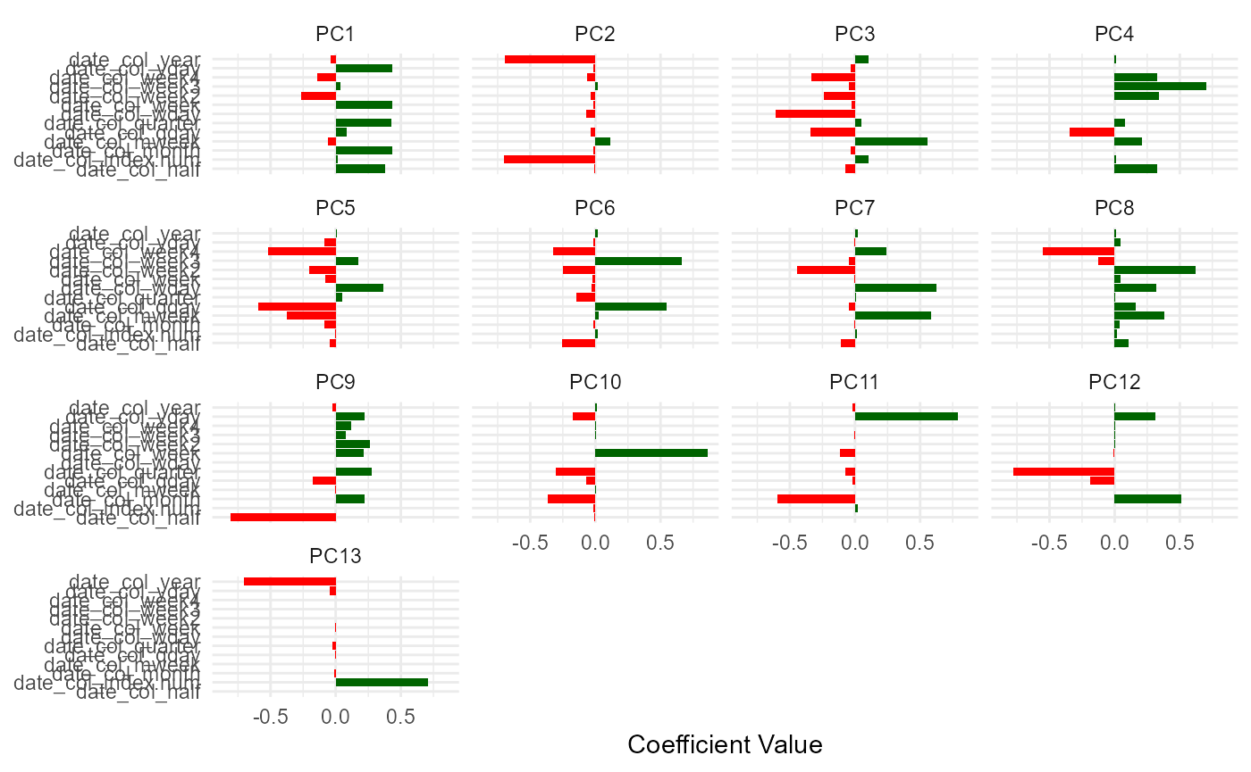
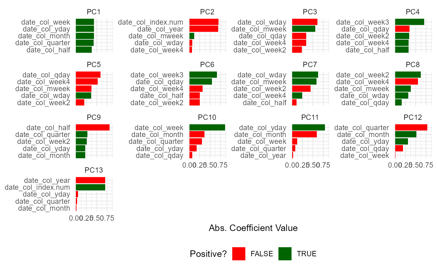
pca_list$pca_rotation_df %>% glimpse()
#> Rows: 13
#> Columns: 13
#> $ PC1  <dbl> 0.016701003, -0.037335907, 0.381058895, 0.429752968, 0.434187301,…
#> $ PC2  <dbl> -0.699632411, -0.697118370, -0.009711570, -0.004442316, -0.012910…
#> $ PC3  <dbl> 0.10269146, 0.10643024, -0.07271158, 0.05071914, -0.03085906, -0.…
#> $ PC4  <dbl> 0.009742488, 0.010284929, 0.324827741, 0.081914474, -0.006010521,…
#> $ PC5  <dbl> -0.004243994, 0.006762025, -0.046625261, 0.051704467, -0.08930171…
#> $ PC6  <dbl> 0.01986614, 0.02143544, -0.25400791, -0.14840873, -0.01599570, -0…
#> $ PC7  <dbl> 0.018042995, 0.018754674, -0.105595683, 0.006701653, -0.004196585…
#> $ PC8  <dbl> 0.019784412, 0.014327818, 0.105805749, 0.001866363, 0.040450916, …
#> $ PC9  <dbl> 0.005222905, -0.022364181, -0.809203933, 0.278940749, 0.221798081…
#> $ PC10 <dbl> -0.013223062, 0.011393666, -0.006386992, -0.304562357, -0.3623196…
#> $ PC11 <dbl> 2.145623e-02, -2.222203e-02, 2.409009e-04, -7.299964e-02, -5.9775…
#> $ PC12 <dbl> -1.847801e-03, 1.525243e-03, -2.943976e-03, -7.776056e-01, 5.1243…
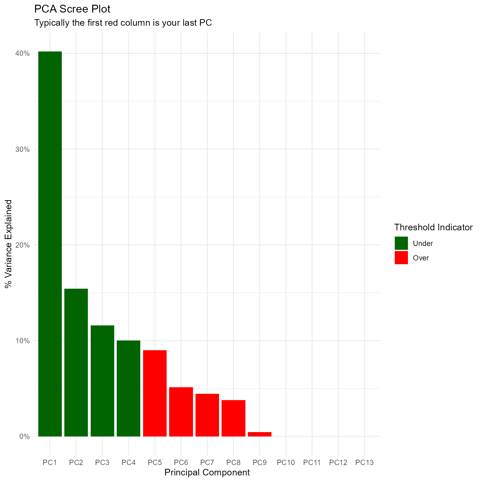
#> $ PC13 <dbl> 7.055491e-01, -7.064067e-01, -9.184277e-05, -2.641426e-02, -8.531…

Variance and Scree Plot

pca_list$pca_variance_df %>% glimpse()
#> Rows: 13
#> Columns: 6
#> $ PC              <chr> "PC1", "PC2", "PC3", "PC4", "PC5", "PC6", "PC7", "PC8"…
#> $ var_explained   <dbl> 4.018983e-01, 1.543031e-01, 1.157904e-01, 1.000044e-01…
#> $ var_pct_txt     <chr> "40.19%", "15.43%", "11.58%", "10.00%", "8.99%", "5.13…
#> $ cum_var_pct     <dbl> 0.4018983, 0.5562014, 0.6719918, 0.7719962, 0.8618845,…
#> $ cum_var_pct_txt <chr> "40.19%", "55.62%", "67.20%", "77.20%", "86.19%", "91.…
#> $ ou_threshold    <fct> Under, Under, Under, Under, Over, Over, Over, Over, Ov…

pca_list$pca_variance_scree_plt

Variable Loading Plots

pca_list$pca_loadings_plt


pca_list$pca_top_n_loadings_plt

A Quick Introduction

Steven P. Sanderson II, MPH

2024-09-11