Time Series Feature Clustering

This function returns an output list of data and plots that come from using the K-Means clustering algorithm on a time series data.

Usage

ts_feature_cluster(
  .data,
  .date_col,
  .value_col,
  ...,
  .features = c("frequency", "entropy", "acf_features"),
  .scale = TRUE,
  .prefix = "ts_",
  .centers = 3
)

Arguments

.data: The data passed must be a data.frame/tibble only.
.date_col: The date column.
.value_col: The column that holds the value of the time series where you want the features and clustering performed on.
...: This is where you can place grouping variables that are passed off to dplyr::group_by()
.features: This is a quoted string vector using c() of features that you would like to pass. You can pass any feature you make or those from the tsfeatures package.
.scale: If TRUE, time series are scaled to mean 0 and sd 1 before features are computed
.prefix: A prefix to prefix the feature columns. Default: "ts_"
.centers: An integer of how many different centers you would like to generate. The default is 3.

Value

A list output

Details

This function will return a list object output. The function itself requires that a time series tibble/data.frame get passed to it, along with the .date_col, the .value_col and a period of data. It uses the underlying function timetk::tk_tsfeatures() and takes the output of that and performs a clustering analysis using the K-Means algorithm.

The function has a parameter of .features which can take any of the features listed in the tsfeatures package by Rob Hyndman. You can also create custom functions in the .GlobalEnviron and it will take them as quoted arguments.

So you can make a function as follows

my_mean <- function(x){return(mean(x, na.rm = TRUE))}

You can then call this by using .features = c("my_mean").

The output of this function includes the following:

Data Section

ts_feature_tbl
user_item_matrix_tbl
mapped_tbl
scree_data_tbl
input_data_tbl (the original data)

Plots

static_plot
plotly_plot

Author

Steven P. Sanderson II, MPH

Examples


library(dplyr)

data_tbl <- ts_to_tbl(AirPassengers) %>%
  mutate(group_id = rep(1:12, 12))

ts_feature_cluster(
  .data = data_tbl,
  .date_col = date_col,
  .value_col = value,
  group_id,
  .features = c("acf_features","entropy"),
  .scale = TRUE,
  .prefix = "ts_",
  .centers = 3
)
#> $data
#> $data$ts_feature_tbl
#> # A tibble: 12 × 8
#>    group_id ts_x_acf1 ts_x_acf10 ts_diff1_acf1 ts_diff1_acf10 ts_diff2_acf1
#>       <int>     <dbl>      <dbl>         <dbl>          <dbl>         <dbl>
#>  1        1     0.741       1.55       -0.0995          0.474       -0.182 
#>  2        2     0.730       1.50       -0.0155          0.654       -0.147 
#>  3        3     0.766       1.62       -0.471           0.562       -0.620 
#>  4        4     0.715       1.46       -0.253           0.457       -0.555 
#>  5        5     0.730       1.48       -0.372           0.417       -0.649 
#>  6        6     0.751       1.61        0.122           0.646        0.0506
#>  7        7     0.745       1.58        0.260           0.236       -0.303 
#>  8        8     0.761       1.60        0.319           0.419       -0.319 
#>  9        9     0.747       1.59       -0.235           0.191       -0.650 
#> 10       10     0.732       1.50       -0.0371          0.269       -0.510 
#> 11       11     0.746       1.54       -0.310           0.357       -0.556 
#> 12       12     0.735       1.51       -0.360           0.294       -0.601 
#> # ℹ 2 more variables: ts_seas_acf1 <dbl>, ts_entropy <dbl>
#> 
#> $data$user_item_matrix_tbl
#> # A tibble: 12 × 8
#>    group_id ts_x_acf1 ts_x_acf10 ts_diff1_acf1 ts_diff1_acf10 ts_diff2_acf1
#>       <int>     <dbl>      <dbl>         <dbl>          <dbl>         <dbl>
#>  1        1     0.741       1.55       -0.0995          0.474       -0.182 
#>  2        2     0.730       1.50       -0.0155          0.654       -0.147 
#>  3        3     0.766       1.62       -0.471           0.562       -0.620 
#>  4        4     0.715       1.46       -0.253           0.457       -0.555 
#>  5        5     0.730       1.48       -0.372           0.417       -0.649 
#>  6        6     0.751       1.61        0.122           0.646        0.0506
#>  7        7     0.745       1.58        0.260           0.236       -0.303 
#>  8        8     0.761       1.60        0.319           0.419       -0.319 
#>  9        9     0.747       1.59       -0.235           0.191       -0.650 
#> 10       10     0.732       1.50       -0.0371          0.269       -0.510 
#> 11       11     0.746       1.54       -0.310           0.357       -0.556 
#> 12       12     0.735       1.51       -0.360           0.294       -0.601 
#> # ℹ 2 more variables: ts_seas_acf1 <dbl>, ts_entropy <dbl>
#> 
#> $data$mapped_tbl
#> # A tibble: 3 × 3
#>   centers k_means  glance          
#>     <int> <list>   <list>          
#> 1       1 <kmeans> <tibble [1 × 4]>
#> 2       2 <kmeans> <tibble [1 × 4]>
#> 3       3 <kmeans> <tibble [1 × 4]>
#> 
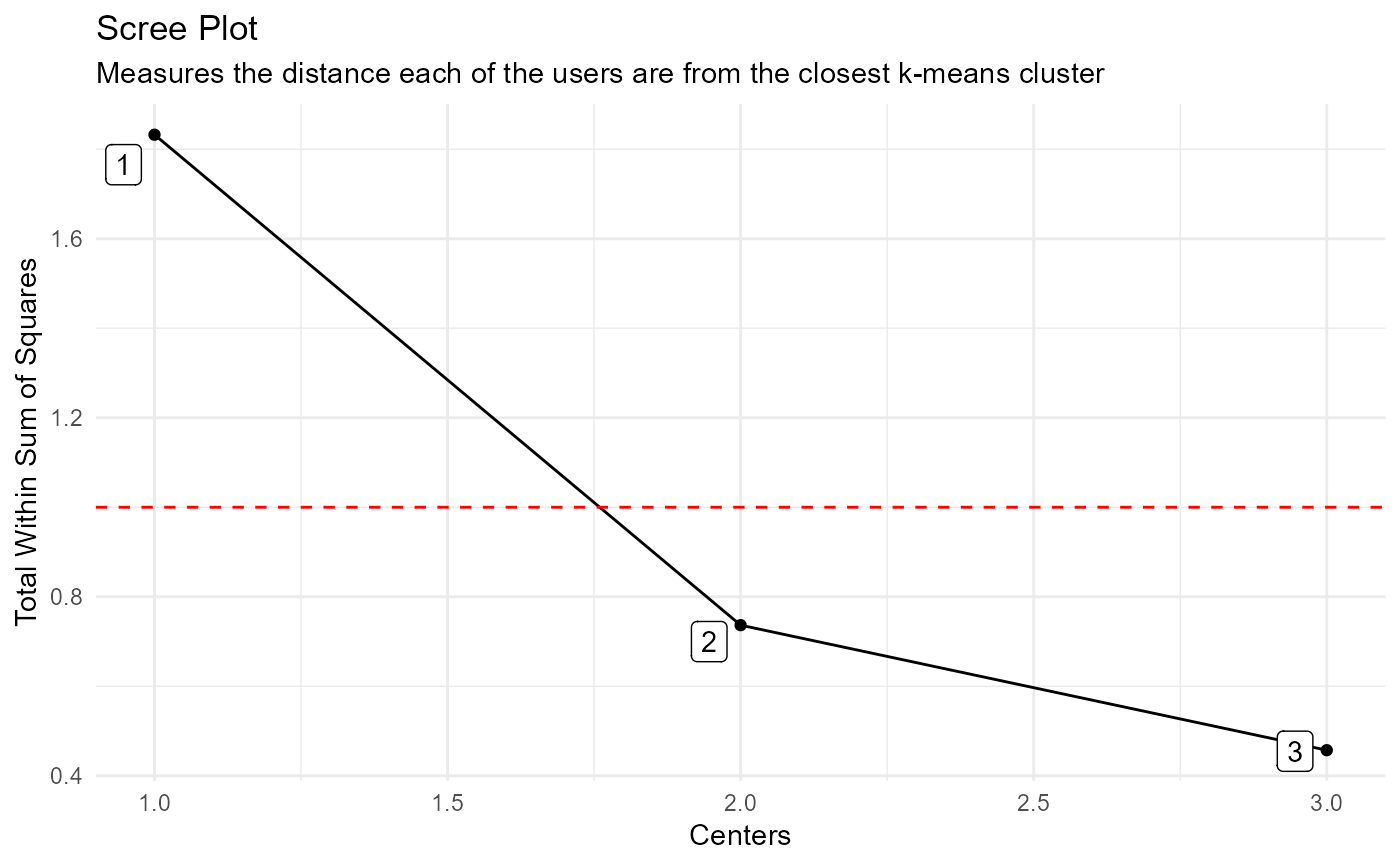
#> $data$scree_data_tbl
#> # A tibble: 3 × 2
#>   centers tot.withinss
#>     <int>        <dbl>
#> 1       1        1.83 
#> 2       2        0.736
#> 3       3        0.457
#> 
#> $data$input_data_tbl
#> # A tibble: 144 × 4
#>    index     date_col   value group_id
#>    <yearmon> <date>     <dbl>    <int>
#>  1 Jan 1949  1949-01-01   112        1
#>  2 Feb 1949  1949-02-01   118        2
#>  3 Mar 1949  1949-03-01   132        3
#>  4 Apr 1949  1949-04-01   129        4
#>  5 May 1949  1949-05-01   121        5
#>  6 Jun 1949  1949-06-01   135        6
#>  7 Jul 1949  1949-07-01   148        7
#>  8 Aug 1949  1949-08-01   148        8
#>  9 Sep 1949  1949-09-01   136        9
#> 10 Oct 1949  1949-10-01   119       10
#> # ℹ 134 more rows
#> 
#> 
#> $plots
#> $plots$static_plot

#> 
#> $plots$plotly_plot
#> 
#> 
#> attr(,"output_type")
#> [1] "ts_feature_cluster"