Time-series Forecasting Simulator

Usage

ts_forecast_simulator(
  .model,
  .data,
  .ext_reg = NULL,
  .frequency = NULL,
  .bootstrap = TRUE,
  .horizon = 4,
  .iterations = 25,
  .sim_color = "steelblue",
  .alpha = 0.05
)

Arguments

.model

A forecasting model of one of the following from the forecast package:

• Arima

• auto.arima

• ets

• nnetar

• Arima() with xreg

.data

The data that is used for the .model parameter. This is used with timetk::tk_index()

.ext_reg

A tibble or matrix of future xregs that should be the same length as the horizon you want to forecast.

.frequency

This is for the conversion of an internal table and should match the time frequency of the data.

.bootstrap

A boolean value of TRUE/FALSE. From forecast::simulate.Arima() Do simulation using resampled errors rather than normally distributed errors.

.horizon

An integer defining the forecast horizon.

.iterations

An integer, set the number of iterations of the simulation.

.sim_color

Set the color of the simulation paths lines.

.alpha

Set the opacity level of the simulation path lines.

Value

The original time series, the simulated values and a some plots

Details

This function expects to take in a model of either Arima, auto.arima, ets or nnetar from the forecast package. You can supply a forecasting horizon, iterations and a few other items. You may also specify an Arima() model using xregs.

See also

Author

Steven P. Sanderson II, MPH

Examples

suppressPackageStartupMessages(library(forecast))
suppressPackageStartupMessages(library(dplyr))

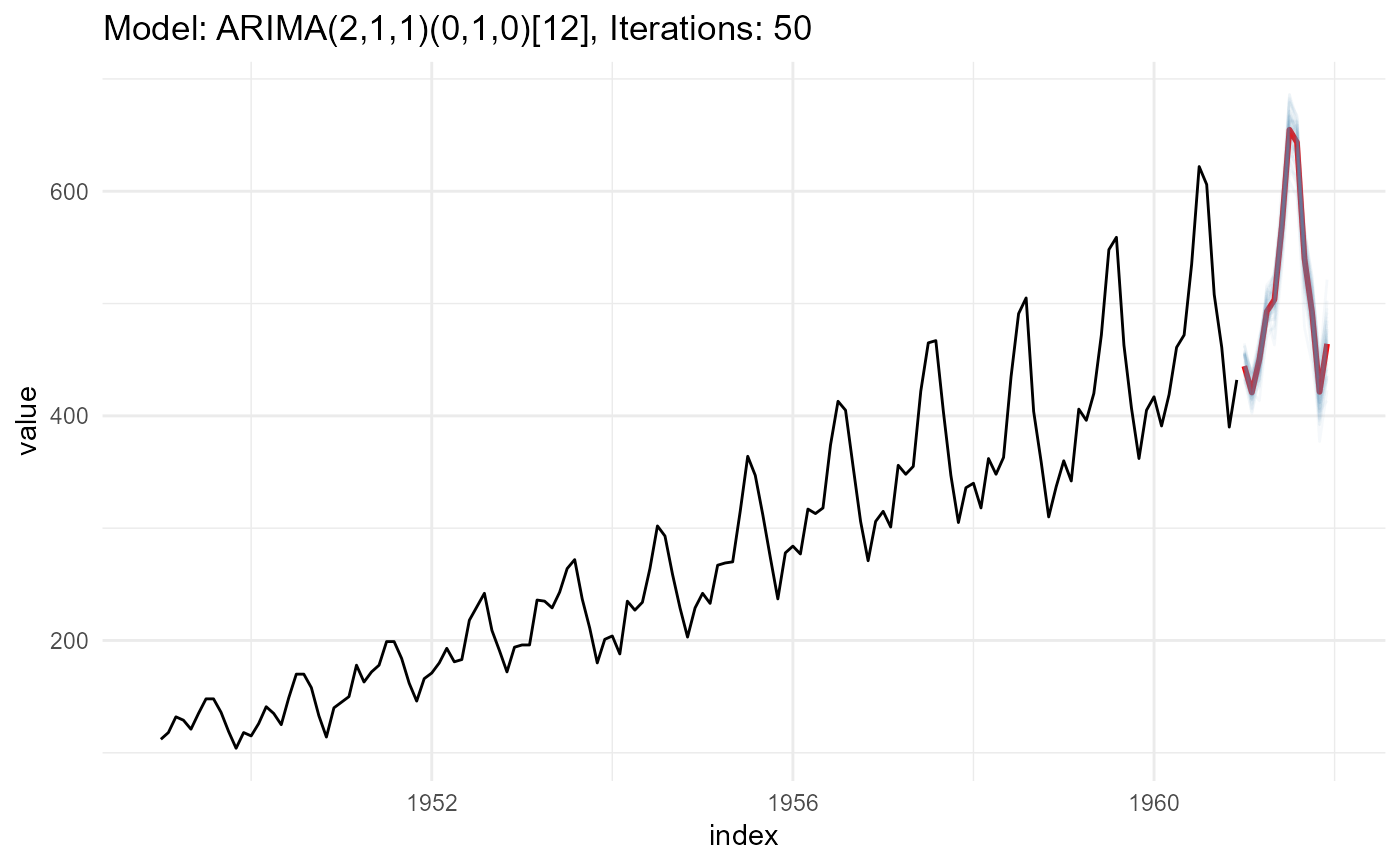
# Create a model
fit <- auto.arima(AirPassengers)
data_tbl <- ts_to_tbl(AirPassengers)

# Simulate 50 possible forecast paths, with .horizon of 12 months
output <- ts_forecast_simulator(
  .model        = fit
  , .horizon    = 12
  , .iterations = 50
  , .data       = data_tbl
)

output$ggplot