healthyverse_tsa
Time Series Analysis, Modeling and Forecasting of the Healthyverse Packages
Steven P. Sanderson II, MPH - Date: 2026-06-15
Introduction
This analysis follows a Nested Modeltime Workflow from modeltime
along with using the NNS package. I use this to monitor the
downloads of all of my packages:
Get Data
glimpse(downloads_tbl)
Rows: 181,317
Columns: 11
$ date      <date> 2020-11-23, 2020-11-23, 2020-11-23, 2020-11-23, 2020-11-23,…
$ time      <Period> 15H 36M 55S, 11H 26M 39S, 23H 34M 44S, 18H 39M 32S, 9H 0M…
$ date_time <dttm> 2020-11-23 15:36:55, 2020-11-23 11:26:39, 2020-11-23 23:34:…
$ size      <int> 4858294, 4858294, 4858301, 4858295, 361, 4863722, 4864794, 4…
$ r_version <chr> NA, "4.0.3", "3.5.3", "3.5.2", NA, NA, NA, NA, NA, NA, NA, N…
$ r_arch    <chr> NA, "x86_64", "x86_64", "x86_64", NA, NA, NA, NA, NA, NA, NA…
$ r_os      <chr> NA, "mingw32", "mingw32", "linux-gnu", NA, NA, NA, NA, NA, N…
$ package   <chr> "healthyR.data", "healthyR.data", "healthyR.data", "healthyR…
$ version   <chr> "1.0.0", "1.0.0", "1.0.0", "1.0.0", "1.0.0", "1.0.0", "1.0.0…
$ country   <chr> "US", "US", "US", "GB", "US", "US", "DE", "HK", "JP", "US", …
$ ip_id     <int> 2069, 2804, 78827, 27595, 90474, 90474, 42435, 74, 7655, 638…
The last day in the data set is 2026-06-13 17:44:04, the file was birthed on: 2025-10-31 10:47:59.603742, and at report knit time is 5402.93 hours old. Happy analyzing!
Now that we have our data lets take a look at it using the skimr
package.
skim(downloads_tbl)
| Name | downloads_tbl |
| Number of rows | 181317 |
| Number of columns | 11 |
| _______________________ | |
| Column type frequency: | |
| character | 6 |
| Date | 1 |
| numeric | 2 |
| POSIXct | 1 |
| Timespan | 1 |
| ________________________ | |
| Group variables | None |
Data summary
Variable type: character
| skim_variable | n_missing | complete_rate | min | max | empty | n_unique | whitespace |
|---|---|---|---|---|---|---|---|
| r_version | 135535 | 0.25 | 5 | 7 | 0 | 51 | 0 |
| r_arch | 135535 | 0.25 | 1 | 7 | 0 | 6 | 0 |
| r_os | 135535 | 0.25 | 7 | 19 | 0 | 30 | 0 |
| package | 0 | 1.00 | 7 | 13 | 0 | 8 | 0 |
| version | 0 | 1.00 | 5 | 17 | 0 | 63 | 0 |
| country | 17216 | 0.91 | 2 | 2 | 0 | 170 | 0 |
Variable type: Date
| skim_variable | n_missing | complete_rate | min | max | median | n_unique |
|---|---|---|---|---|---|---|
| date | 0 | 1 | 2020-11-23 | 2026-06-13 | 2024-01-27 | 2022 |
Variable type: numeric
| skim_variable | n_missing | complete_rate | mean | sd | p0 | p25 | p50 | p75 | p100 | hist |
|---|---|---|---|---|---|---|---|---|---|---|
| size | 0 | 1 | 1131371.30 | 1475488.95 | 355 | 43637 | 325577 | 2334107 | 5677952 | ▇▁▂▁▁ |
| ip_id | 0 | 1 | 11824.26 | 24283.72 | 1 | 168 | 2711 | 11874 | 299146 | ▇▁▁▁▁ |
Variable type: POSIXct
| skim_variable | n_missing | complete_rate | min | max | median | n_unique |
|---|---|---|---|---|---|---|
| date_time | 0 | 1 | 2020-11-23 09:00:41 | 2026-06-13 17:44:04 | 2024-01-27 01:26:46 | 115806 |
Variable type: Timespan
| skim_variable | n_missing | complete_rate | min | max | median | n_unique |
|---|---|---|---|---|---|---|
| time | 0 | 1 | 0 | 59 | 12H 11M 40S | 60 |
We can see that the following columns are missing a lot of data and for
us are most likely not useful anyways, so we will drop them
c(r_version, r_arch, r_os)
Plots
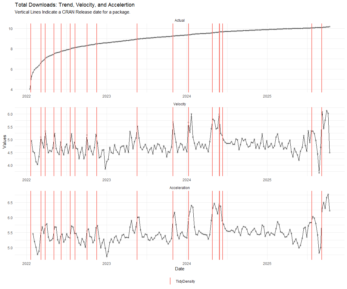
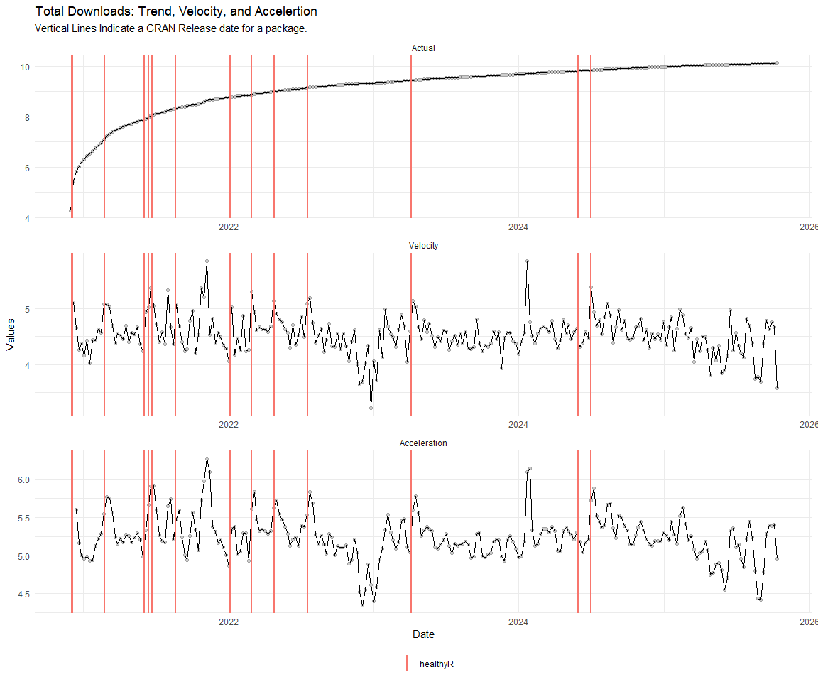
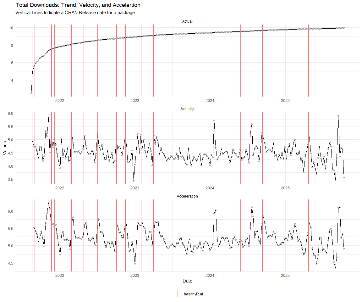
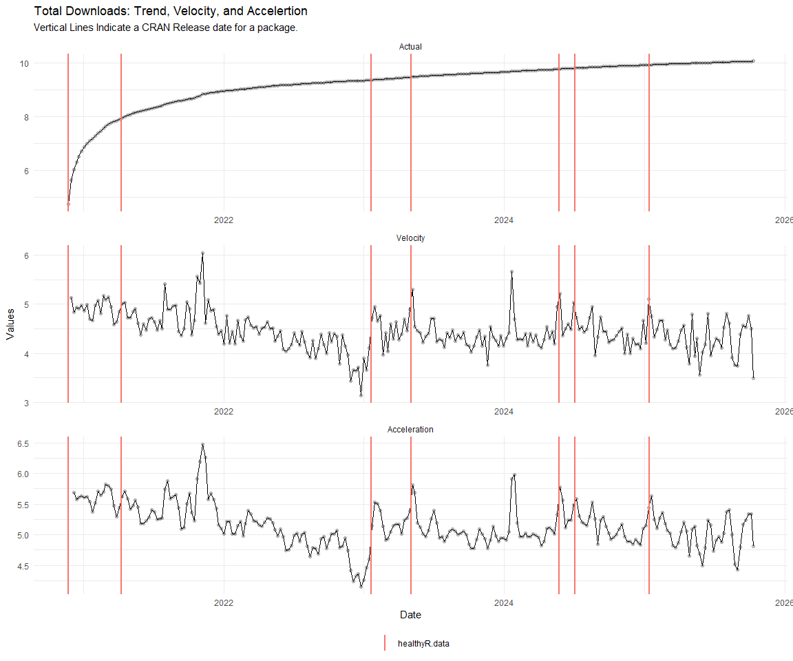
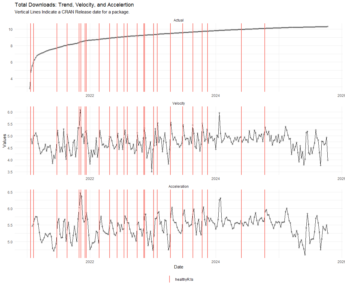
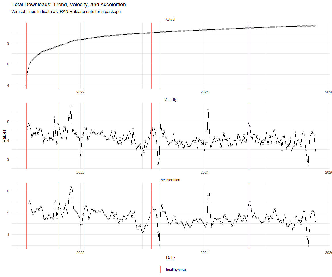
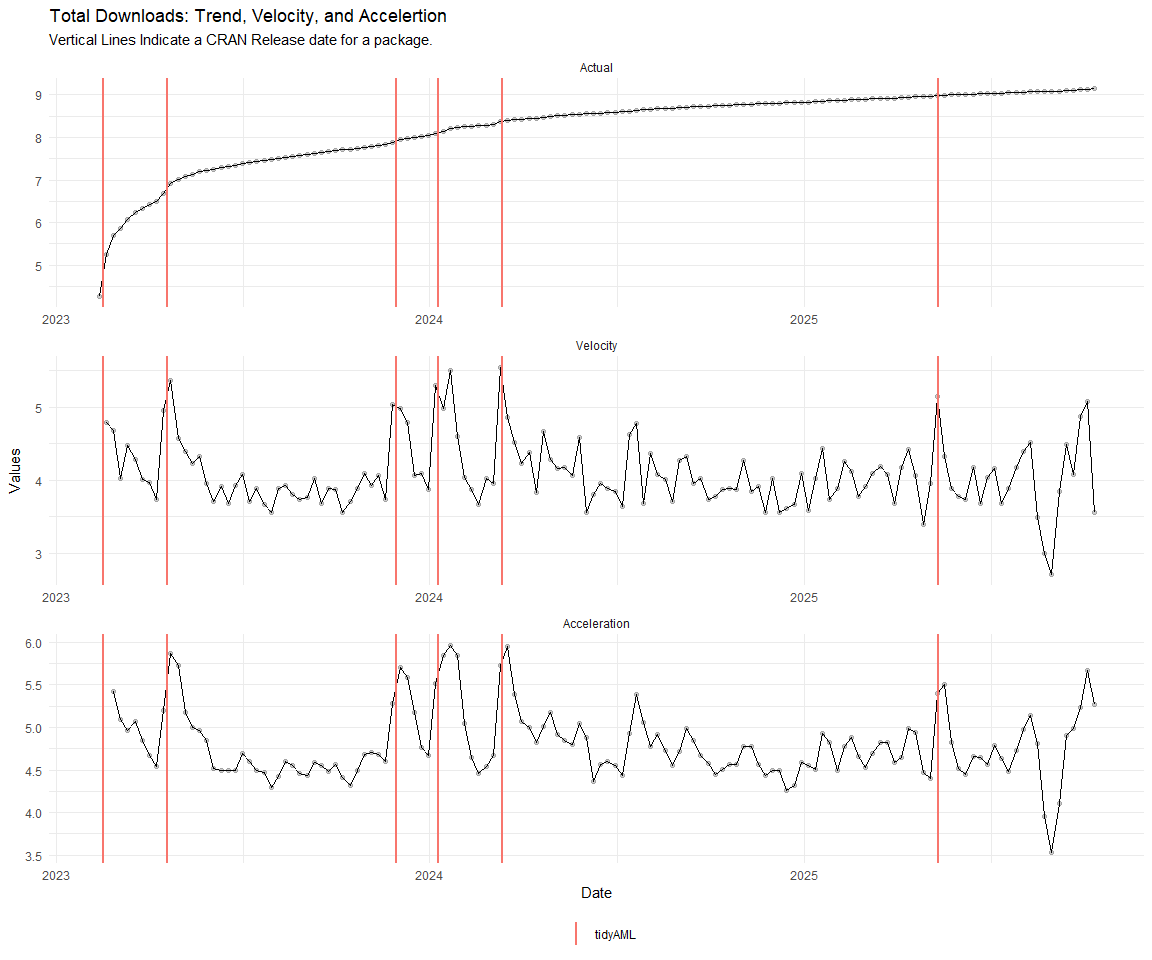
Now lets take a look at a time-series plot of the total daily downloads by package. We will use a log scale and place a vertical line at each version release for each package.
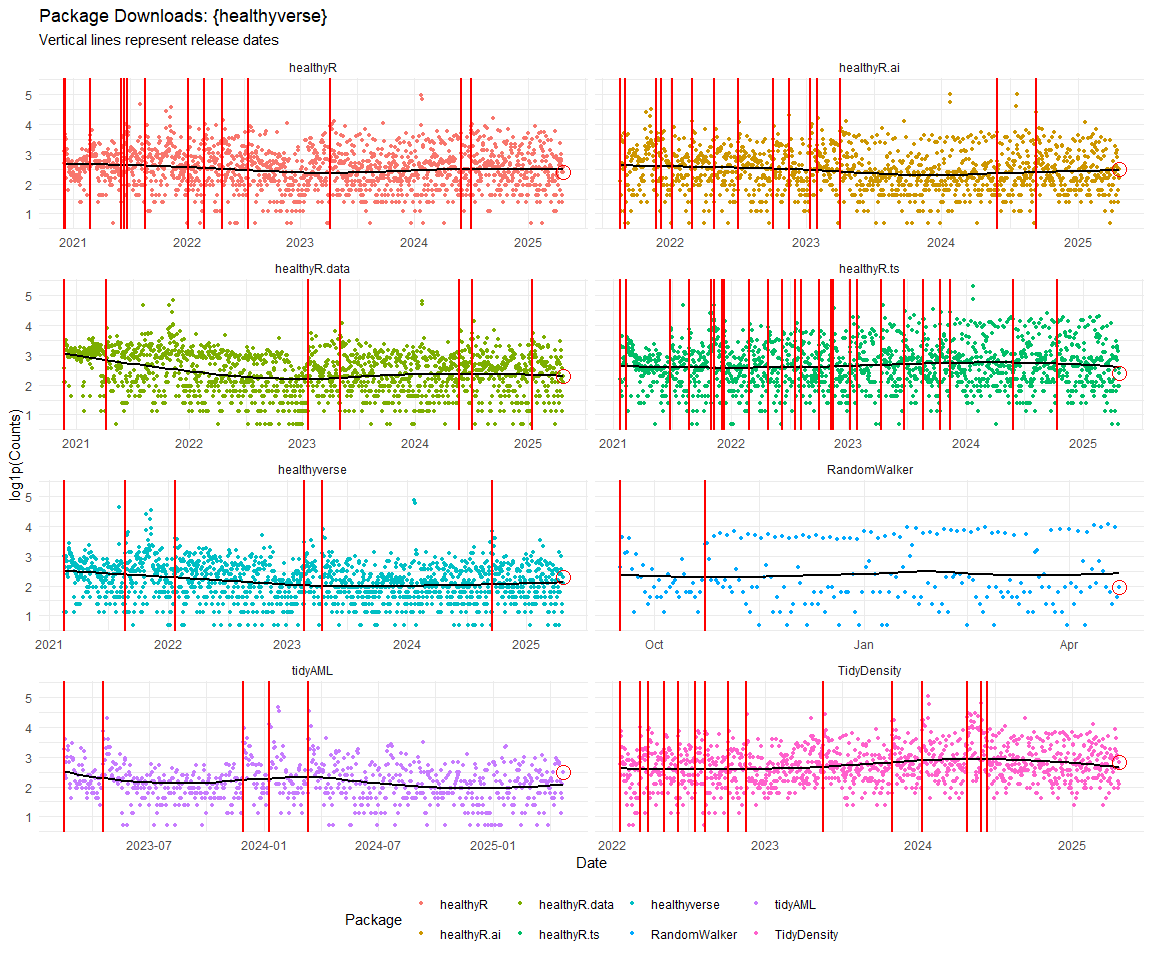
[[1]]
[[2]]
[[3]]
[[4]]
[[5]]
[[6]]
[[7]]
[[8]]
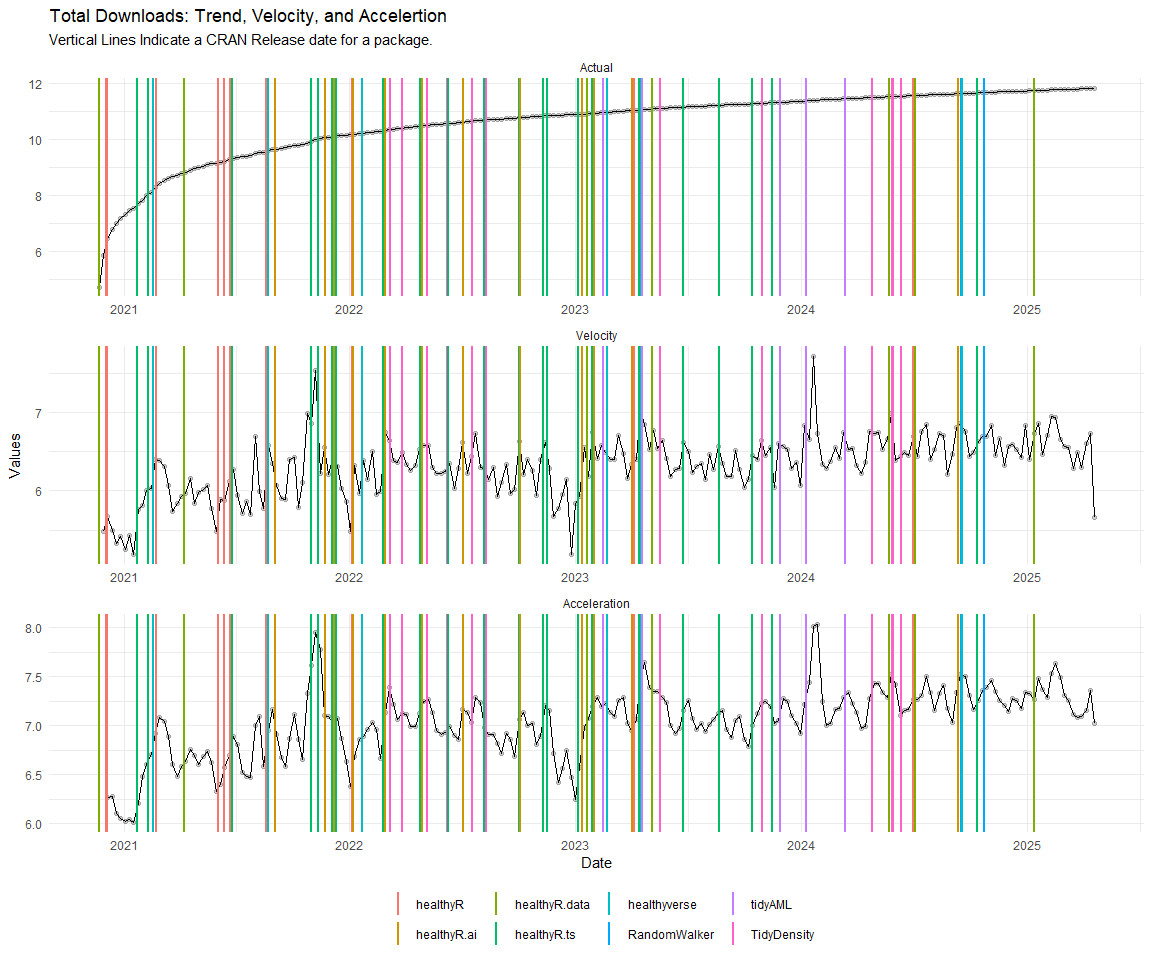
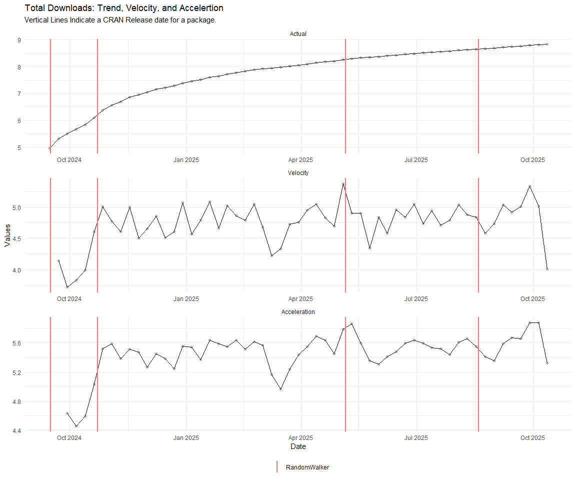
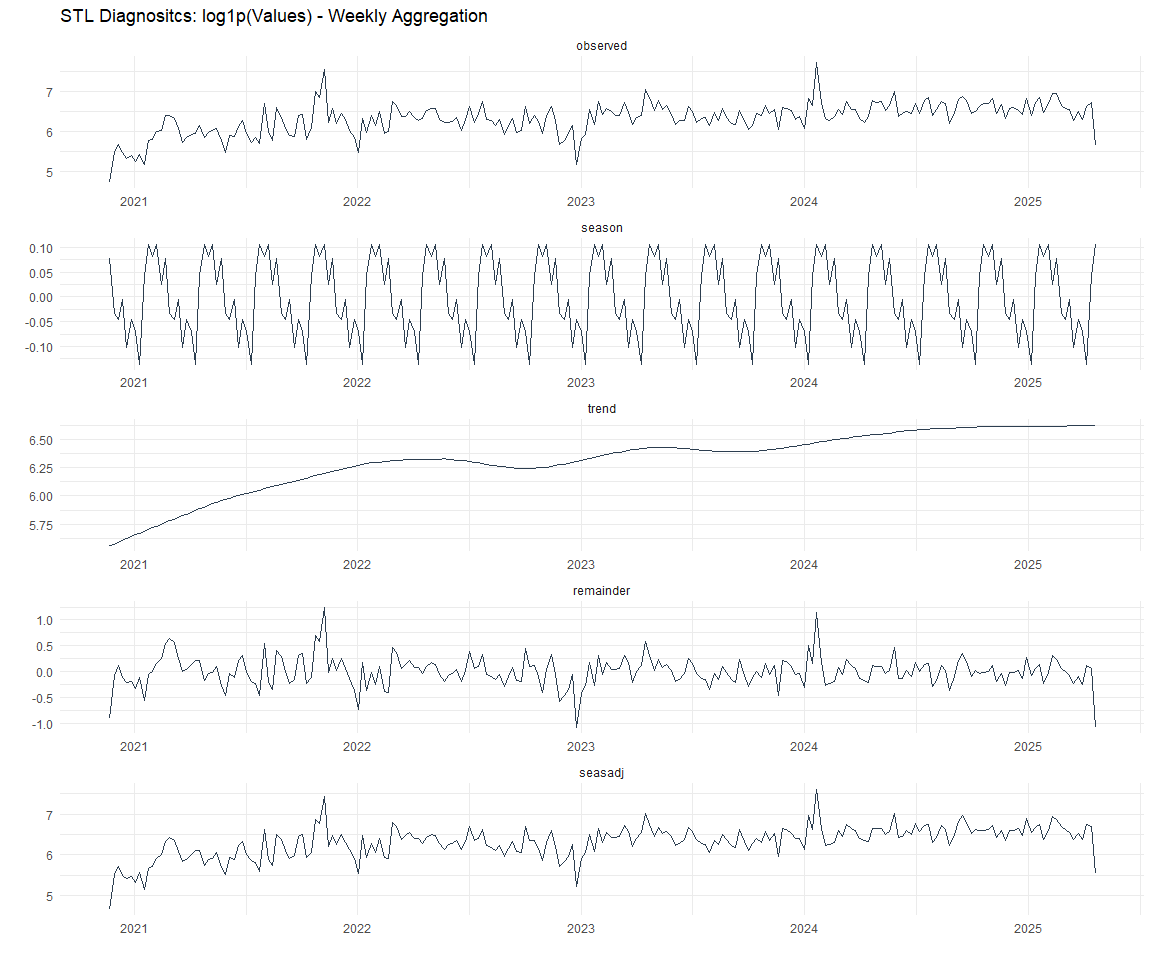
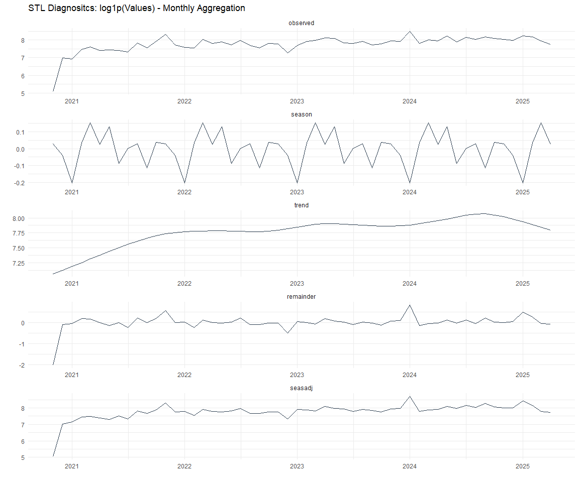
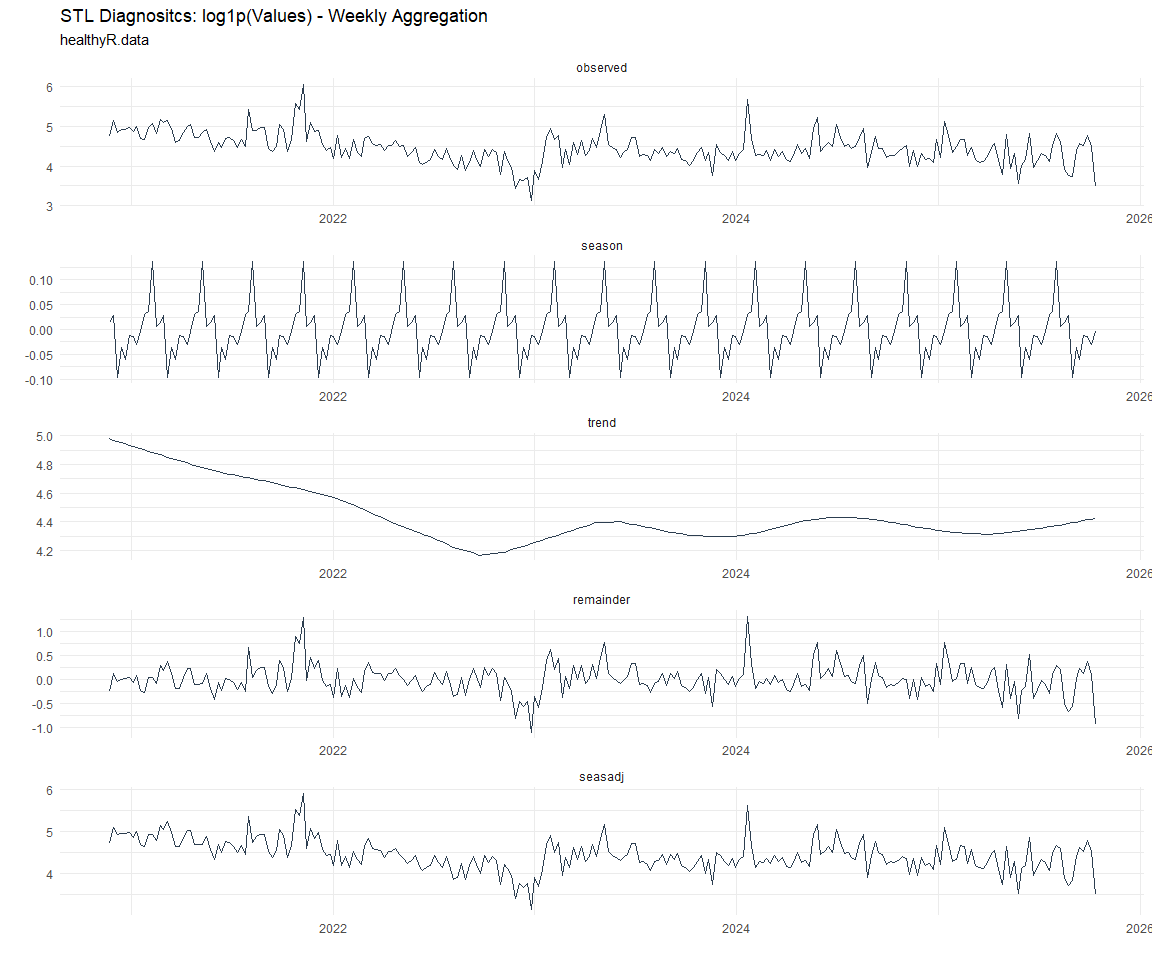
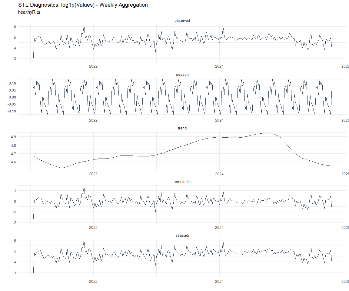
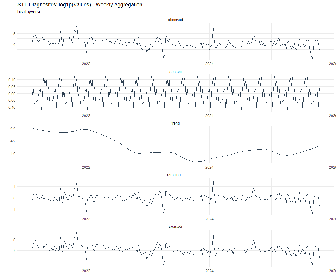
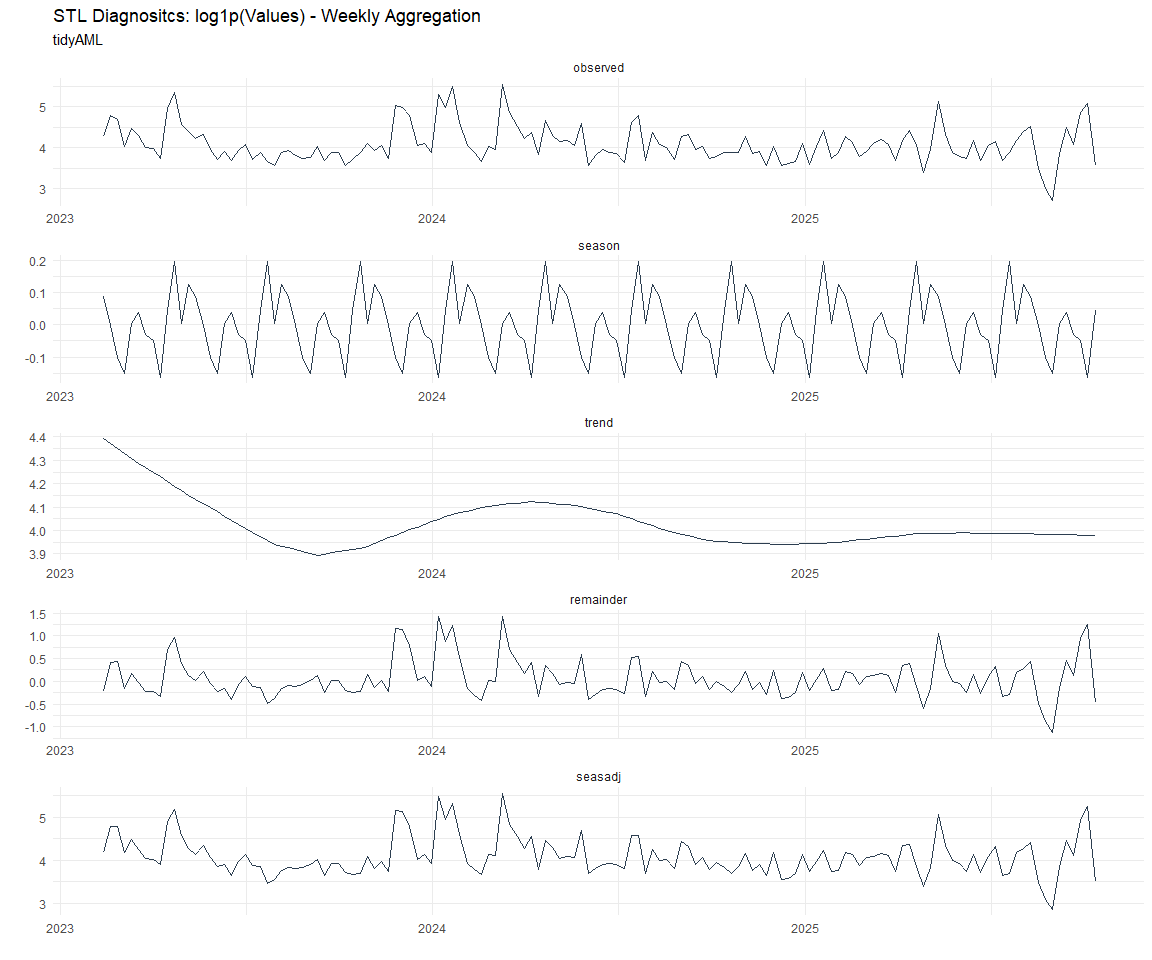
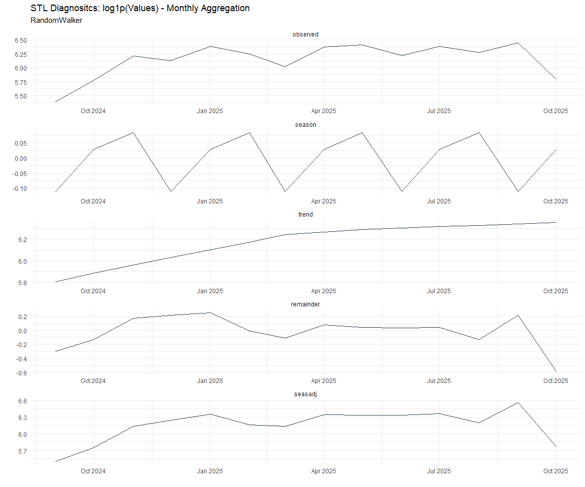
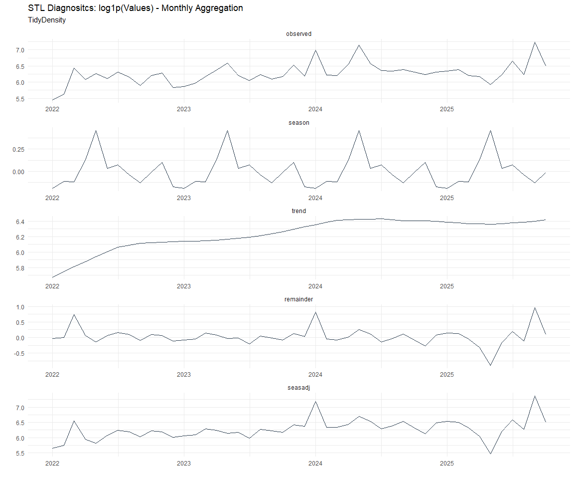
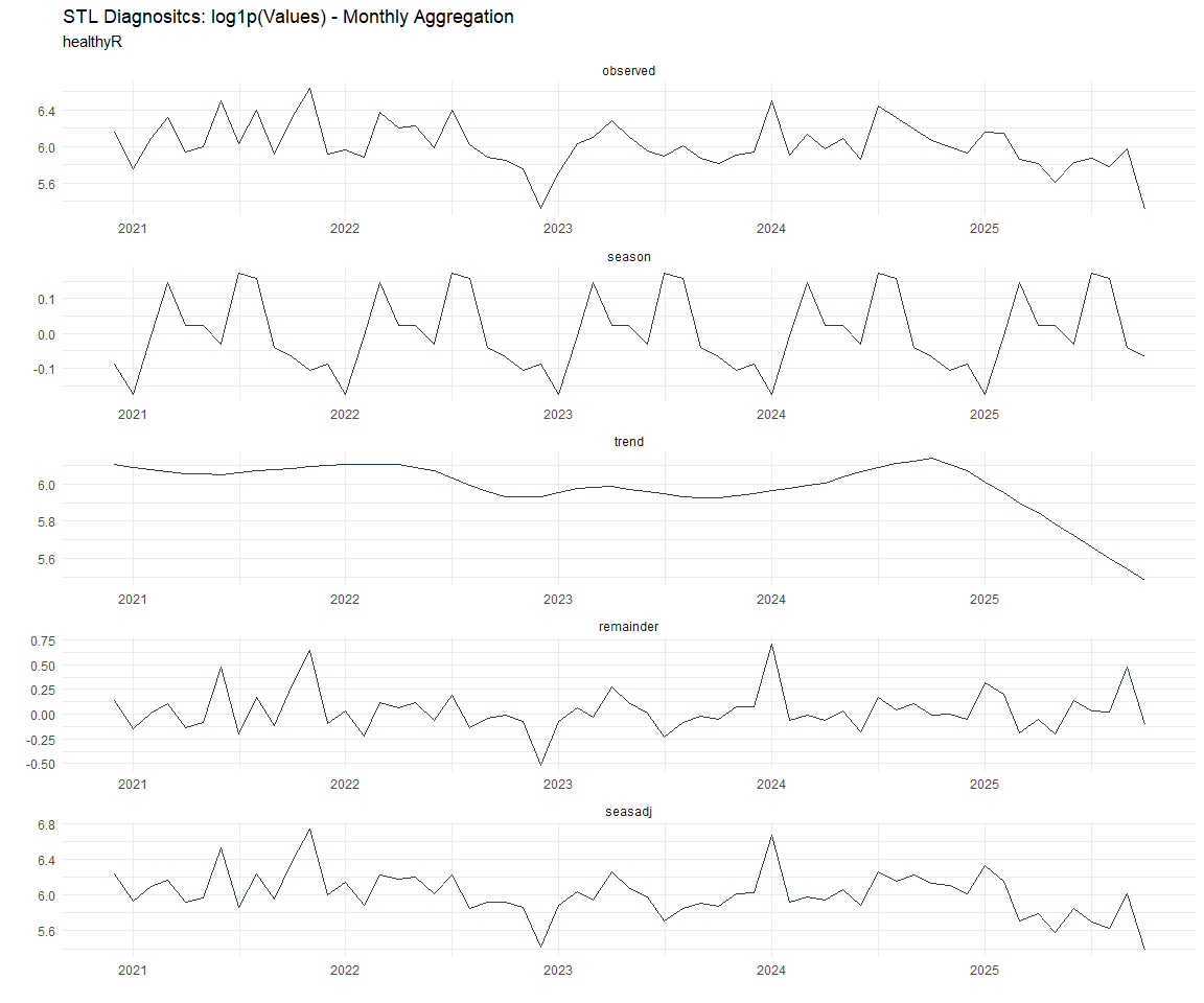
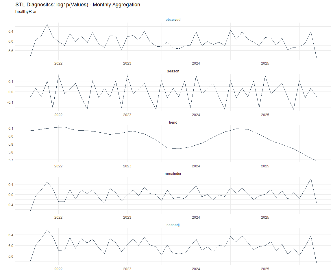
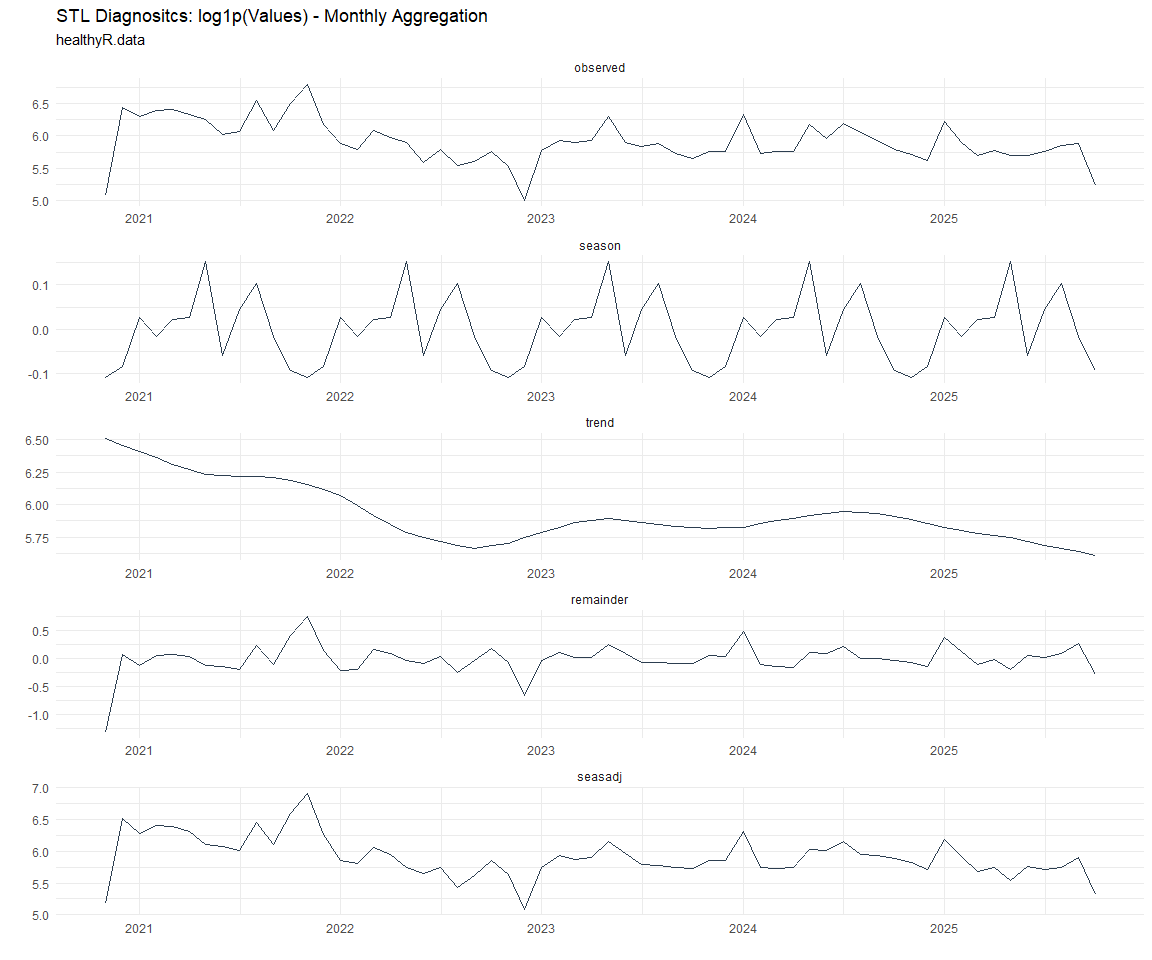
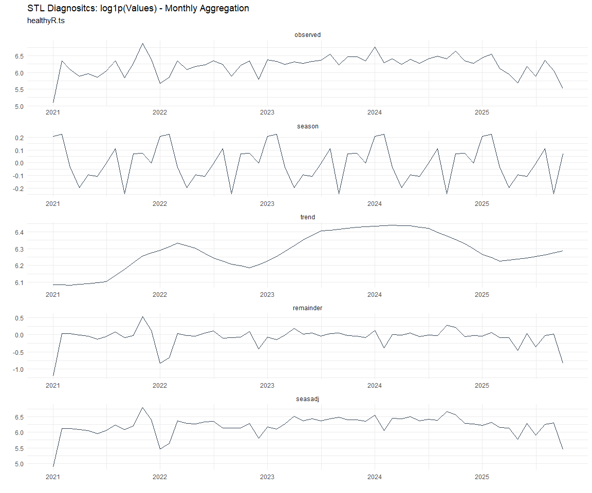
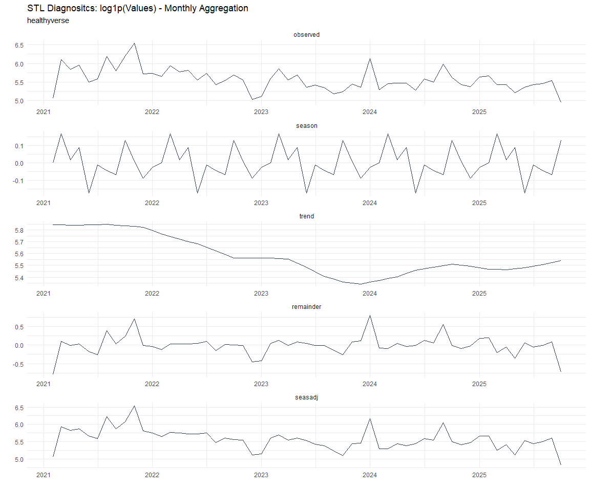
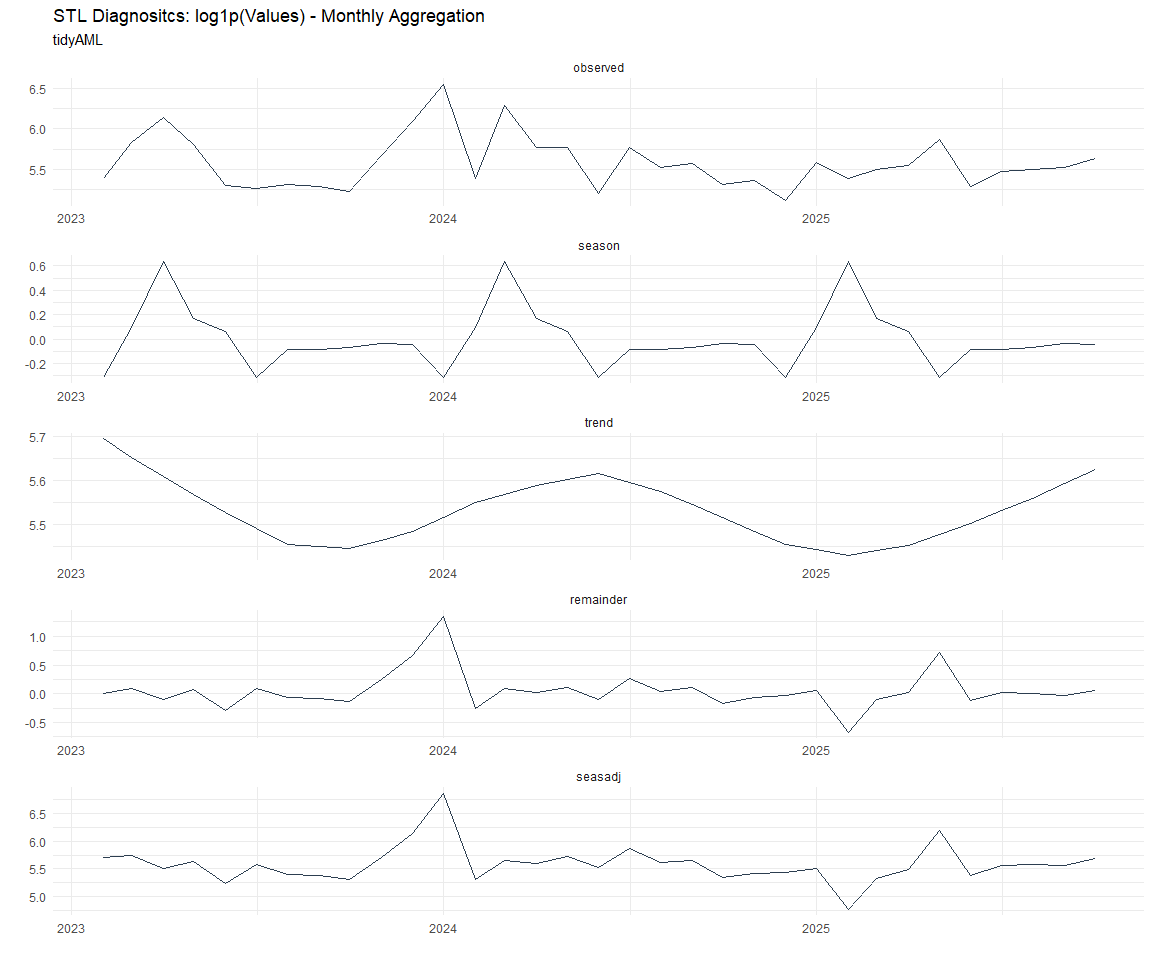
Now lets take a look at some time series decomposition graphs.
[[1]]
[[2]]
[[3]]
[[4]]
[[5]]
[[6]]
[[7]]
[[8]]
[[1]]
[[2]]
[[3]]
[[4]]
[[5]]
[[6]]
[[7]]
[[8]]
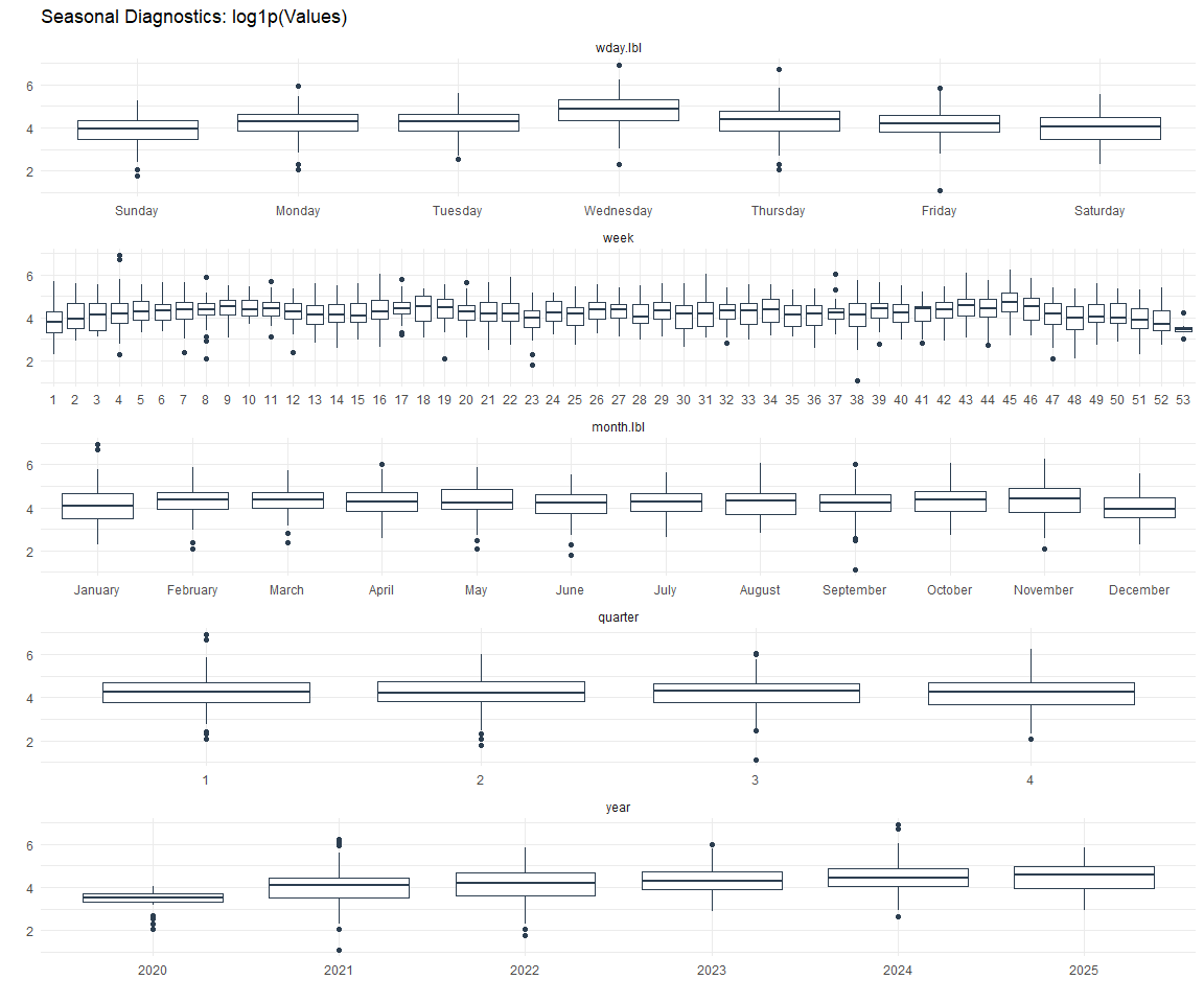
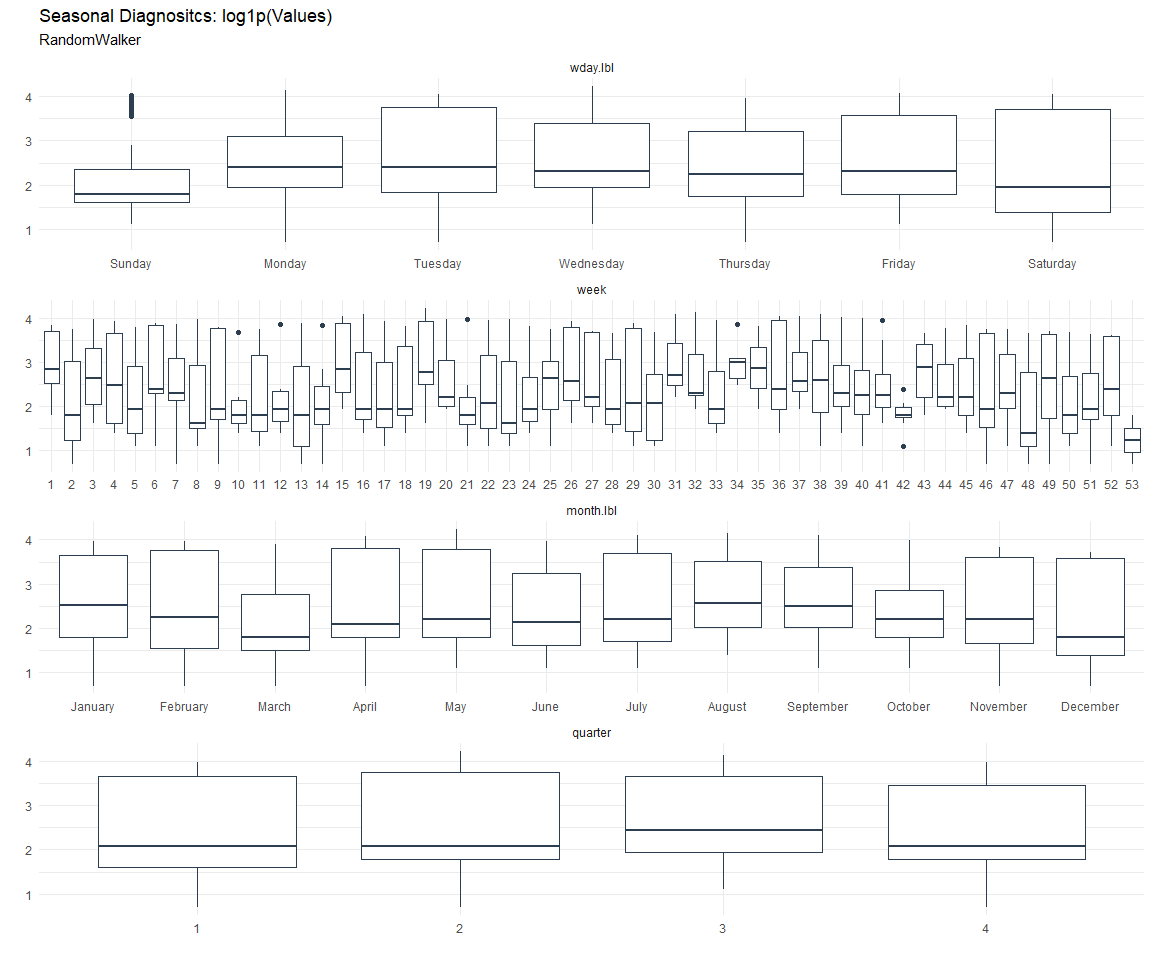
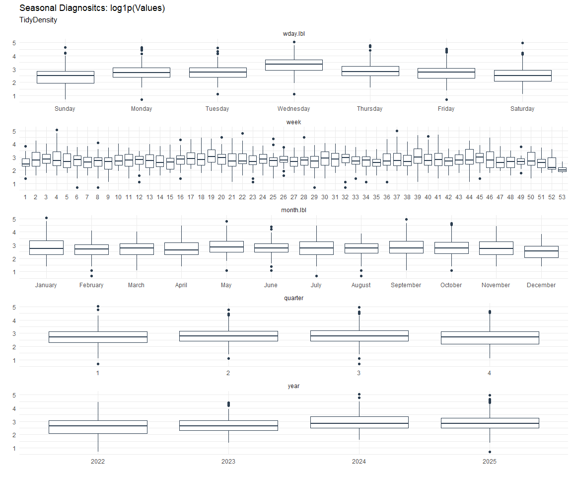
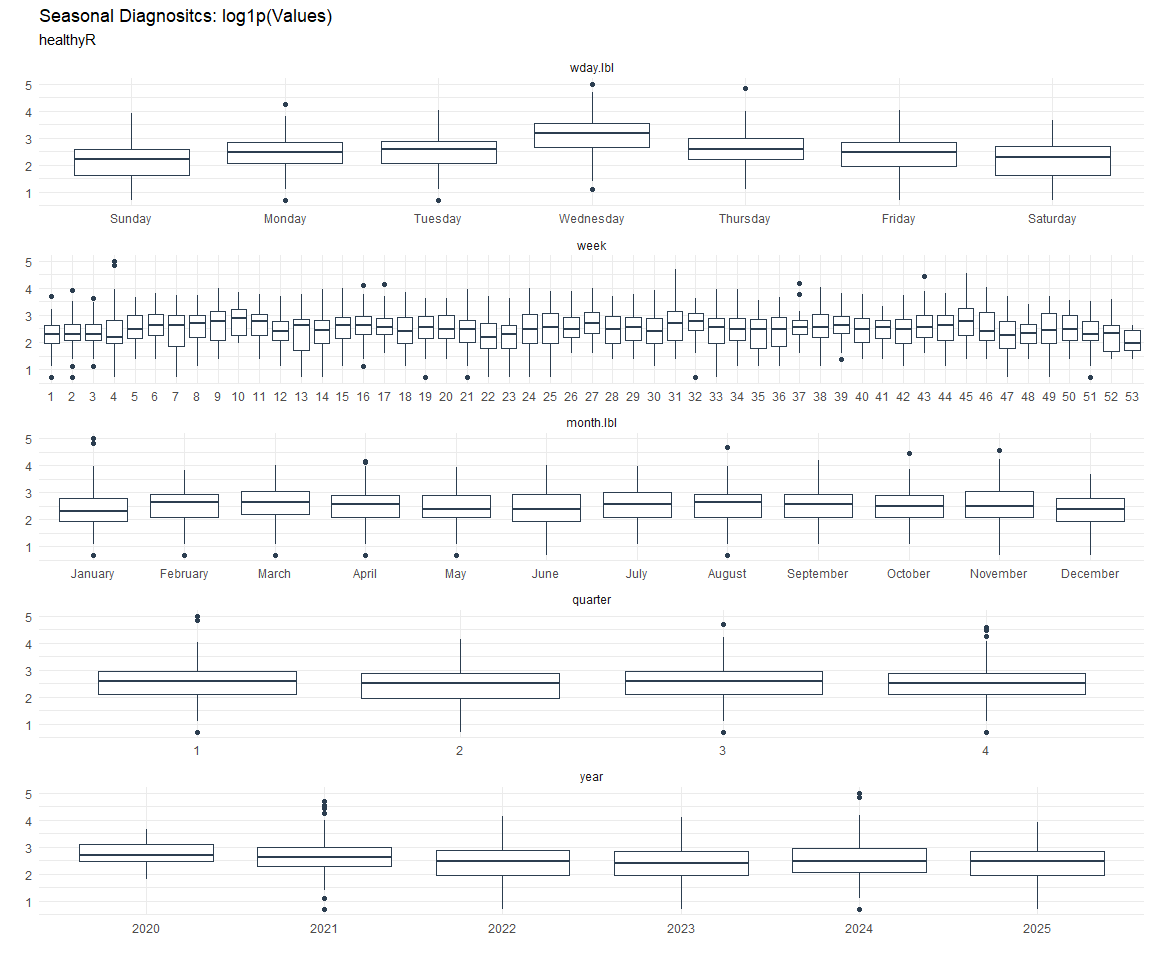
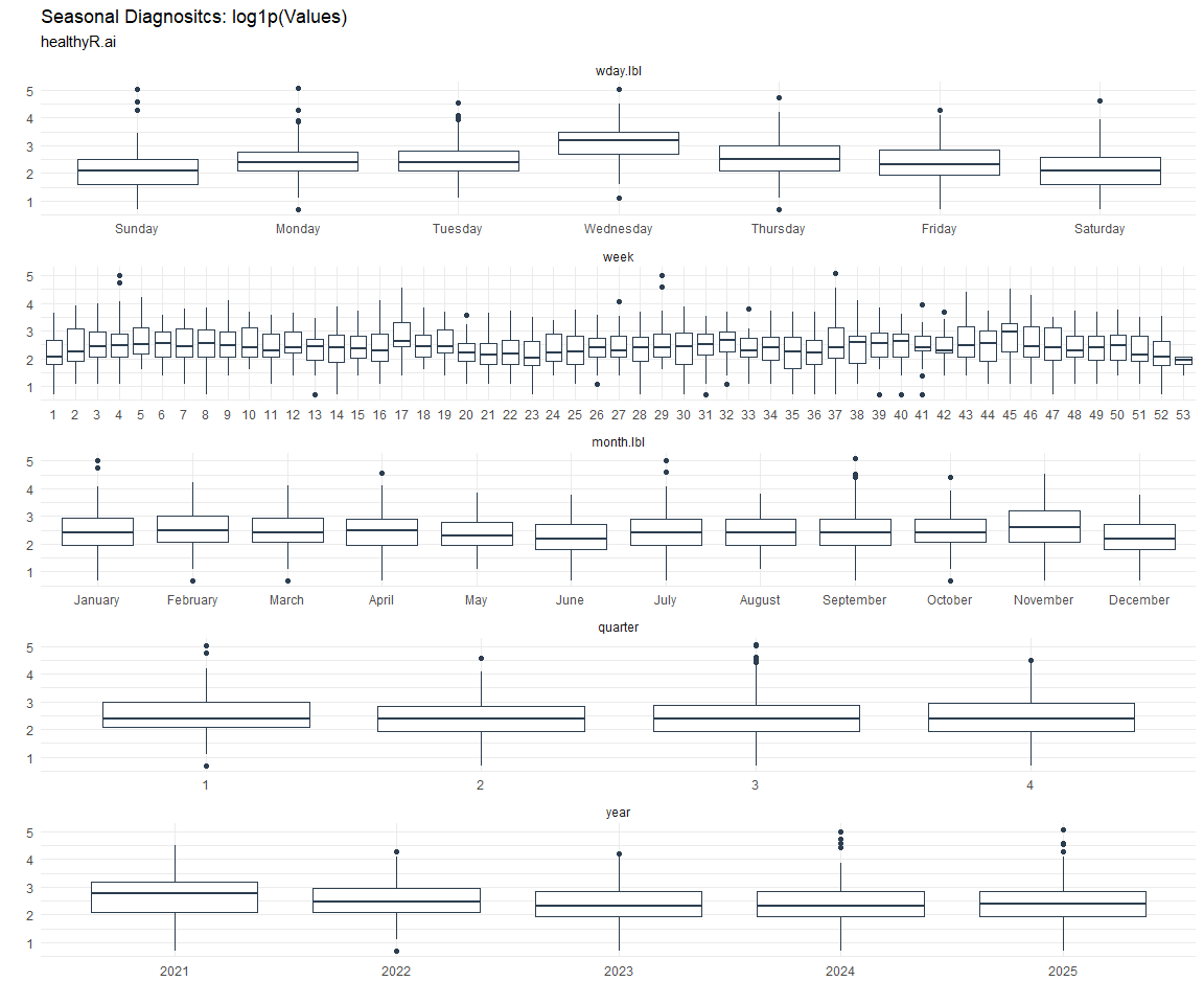
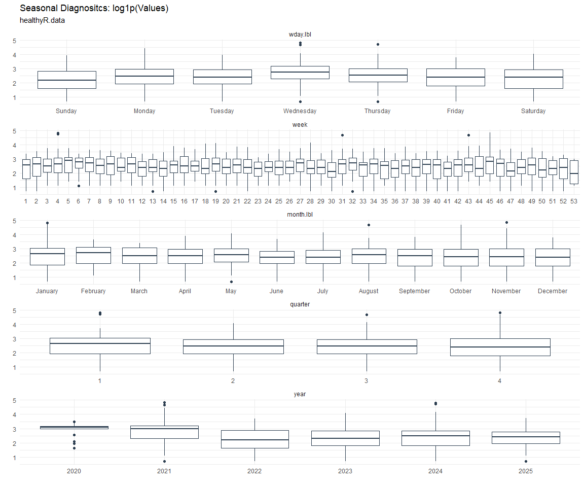
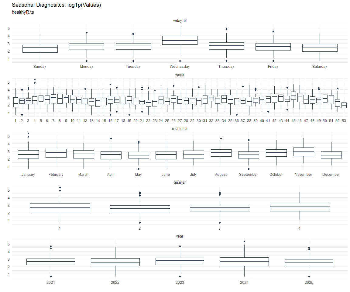
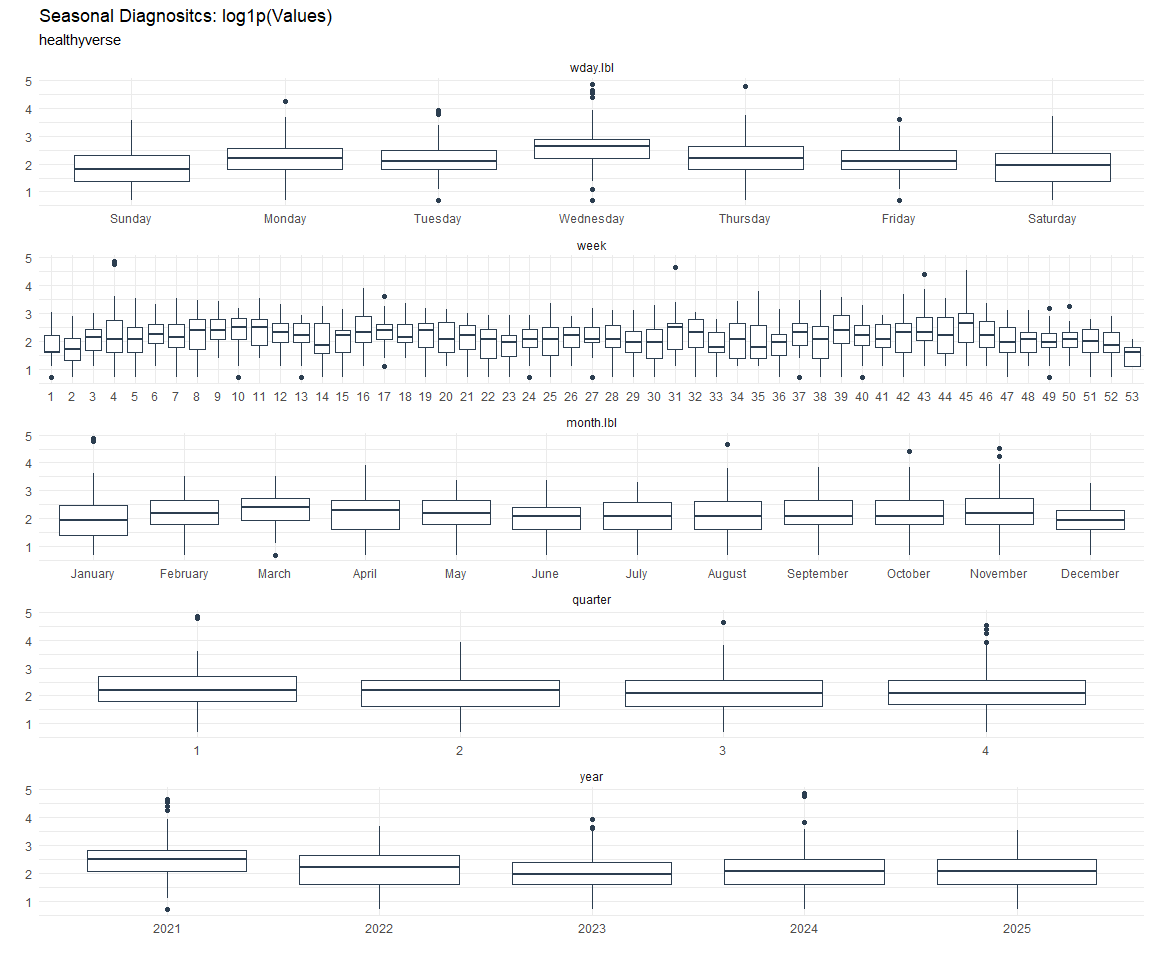
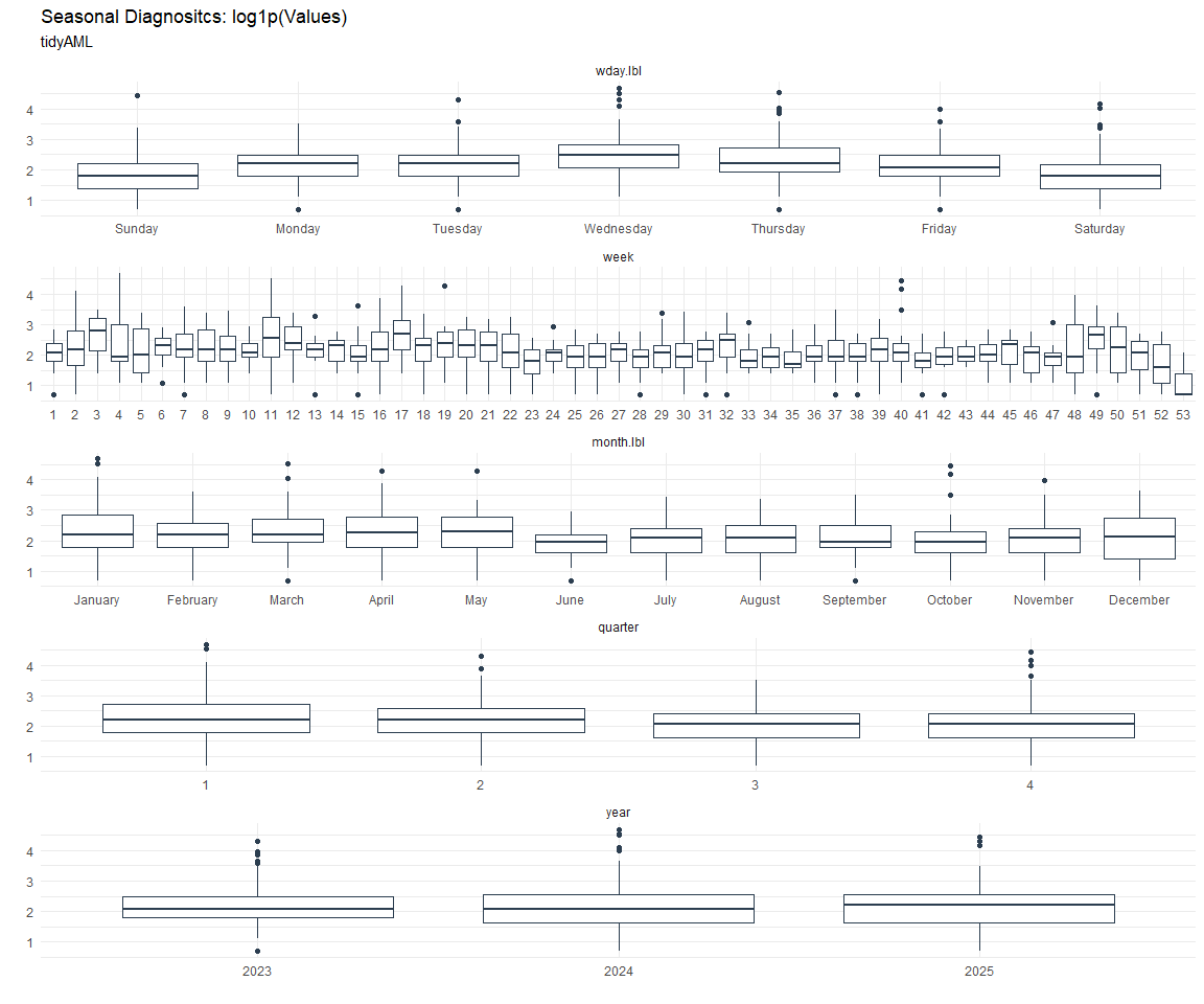
Seasonal Diagnostics:
[[1]]
[[2]]
[[3]]
[[4]]
[[5]]
[[6]]
[[7]]
[[8]]
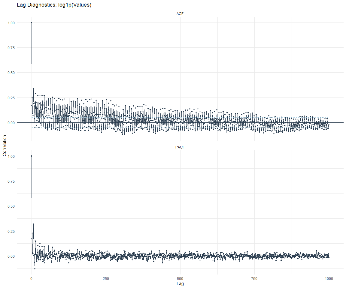
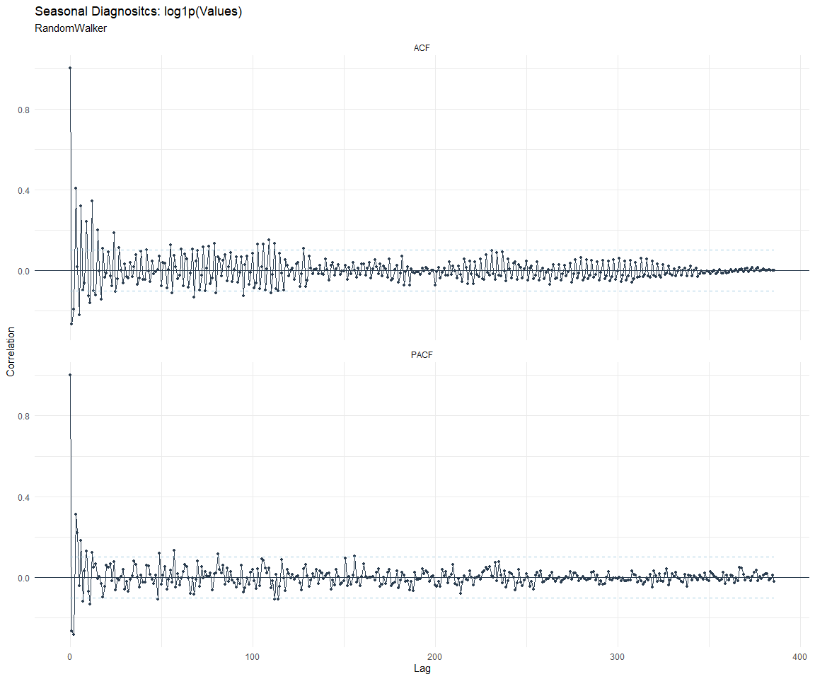
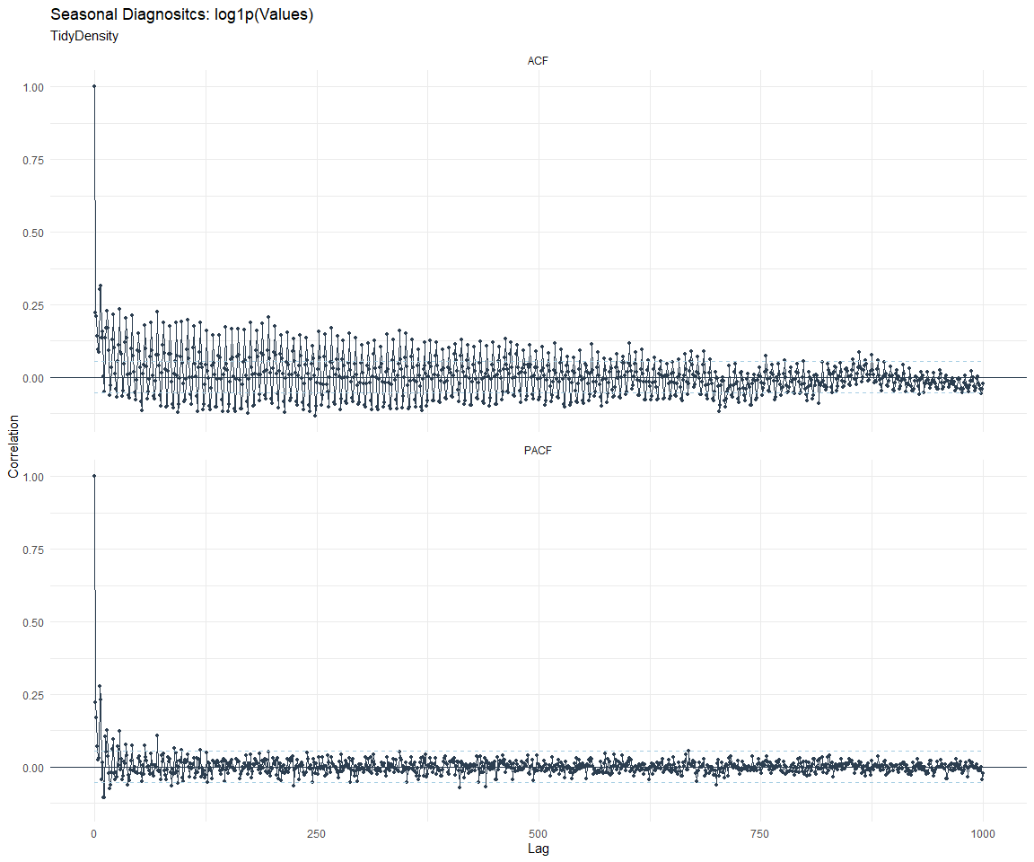
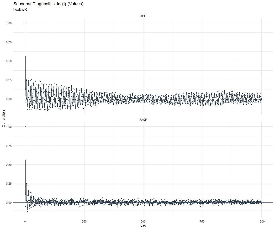
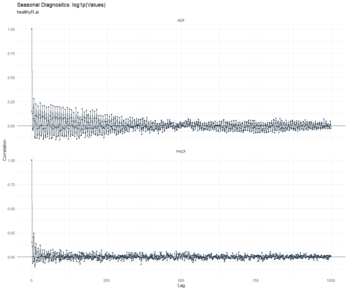
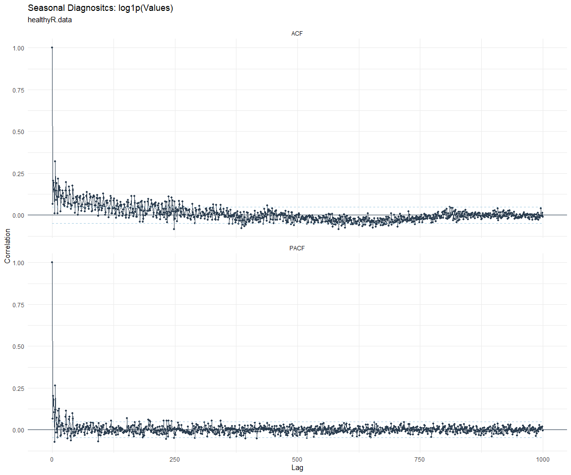
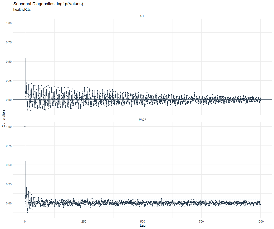
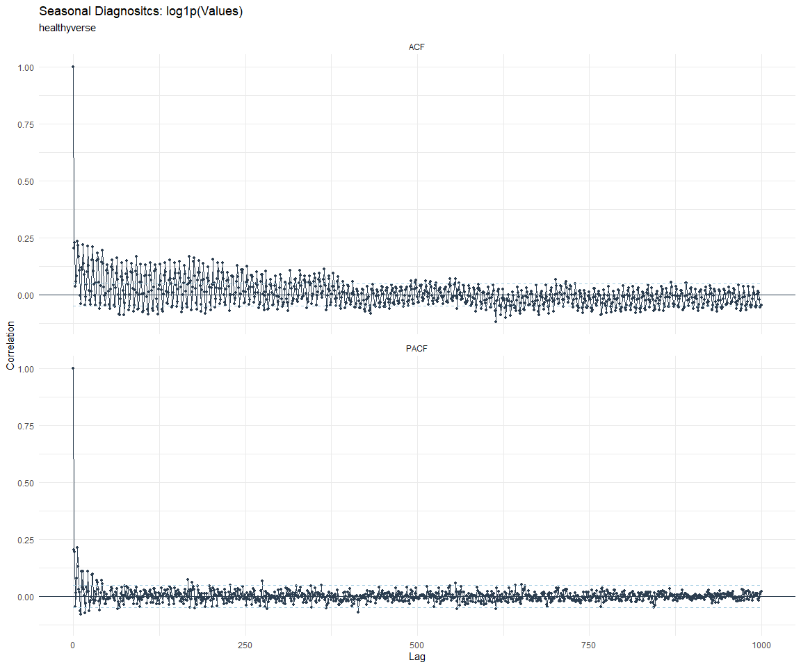
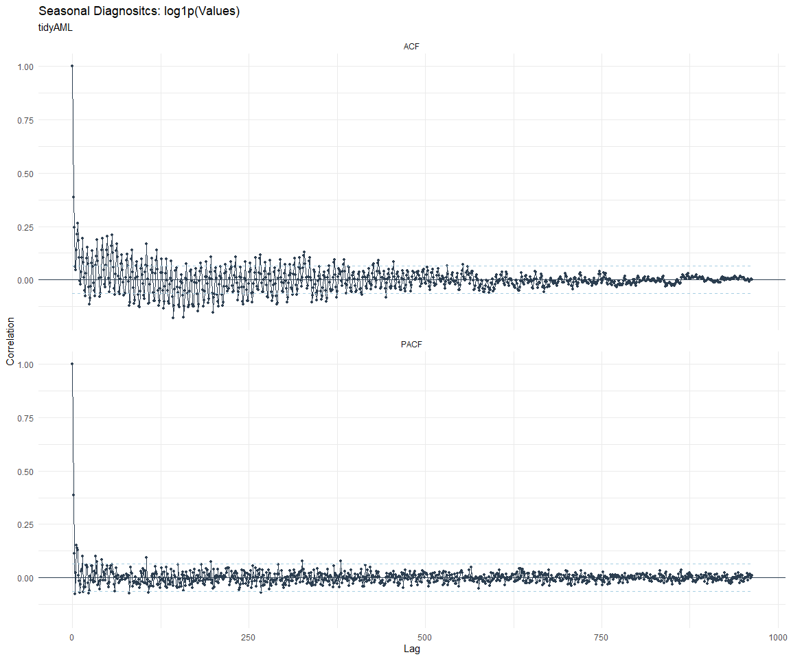
ACF and PACF Diagnostics:
[[1]]
[[2]]
[[3]]
[[4]]
[[5]]
[[6]]
[[7]]
[[8]]
Feature Engineering
Now that we have our basic data and a shot of what it looks like, let’s
add some features to our data which can be very helpful in modeling.
Lets start by making a tibble that is aggregated by the day and
package, as we are going to be interested in forecasting the next 4
weeks or 28 days for each package. First lets get our base data.
Call:
stats::lm(formula = .formula, data = df)

Residuals:
    Min      1Q  Median      3Q     Max
-151.55  -37.83  -11.67   28.67  828.66

Coefficients:
                                                     Estimate Std. Error
(Intercept)                                        -1.659e+02  5.119e+01
date                                                1.048e-02  2.706e-03
lag(value, 1)                                       8.704e-02  2.226e-02
lag(value, 7)                                       7.298e-02  2.287e-02
lag(value, 14)                                      6.782e-02  2.275e-02
lag(value, 21)                                      8.792e-02  2.281e-02
lag(value, 28)                                      7.485e-02  2.273e-02
lag(value, 35)                                      4.133e-02  2.276e-02
lag(value, 42)                                      6.239e-02  2.286e-02
lag(value, 49)                                      7.424e-02  2.280e-02
month(date, label = TRUE).L                        -8.366e+00  4.741e+00
month(date, label = TRUE).Q                        -4.253e-01  4.713e+00
month(date, label = TRUE).C                        -1.589e+01  4.723e+00
month(date, label = TRUE)^4                        -7.961e+00  4.768e+00
month(date, label = TRUE)^5                        -4.073e+00  4.731e+00
month(date, label = TRUE)^6                        -1.864e+00  4.769e+00
month(date, label = TRUE)^7                        -3.982e+00  4.705e+00
month(date, label = TRUE)^8                        -3.024e+00  4.690e+00
month(date, label = TRUE)^9                         2.110e+00  4.713e+00
month(date, label = TRUE)^10                       -2.135e-01  4.712e+00
month(date, label = TRUE)^11                       -2.287e+00  4.752e+00
fourier_vec(date, type = "sin", K = 1, period = 7) -1.109e+01  2.115e+00
fourier_vec(date, type = "cos", K = 1, period = 7)  7.678e+00  2.176e+00
                                                   t value Pr(>|t|)
(Intercept)                                         -3.241 0.001211 **
date                                                 3.873 0.000111 ***
lag(value, 1)                                        3.910 9.54e-05 ***
lag(value, 7)                                        3.191 0.001442 **
lag(value, 14)                                       2.982 0.002901 **
lag(value, 21)                                       3.854 0.000120 ***
lag(value, 28)                                       3.293 0.001009 **
lag(value, 35)                                       1.817 0.069445 .
lag(value, 42)                                       2.730 0.006395 **
lag(value, 49)                                       3.256 0.001148 **
month(date, label = TRUE).L                         -1.765 0.077776 .
month(date, label = TRUE).Q                         -0.090 0.928099
month(date, label = TRUE).C                         -3.364 0.000782 ***
month(date, label = TRUE)^4                         -1.670 0.095098 .
month(date, label = TRUE)^5                         -0.861 0.389369
month(date, label = TRUE)^6                         -0.391 0.695876
month(date, label = TRUE)^7                         -0.846 0.397461
month(date, label = TRUE)^8                         -0.645 0.519199
month(date, label = TRUE)^9                          0.448 0.654504
month(date, label = TRUE)^10                        -0.045 0.963867
month(date, label = TRUE)^11                        -0.481 0.630394
fourier_vec(date, type = "sin", K = 1, period = 7)  -5.244 1.74e-07 ***
fourier_vec(date, type = "cos", K = 1, period = 7)   3.528 0.000429 ***
---
Signif. codes:  0 '***' 0.001 '**' 0.01 '*' 0.05 '.' 0.1 ' ' 1

Residual standard error: 60.12 on 1950 degrees of freedom
  (49 observations deleted due to missingness)
Multiple R-squared:  0.204, Adjusted R-squared:  0.195
F-statistic: 22.71 on 22 and 1950 DF,  p-value: < 2.2e-16
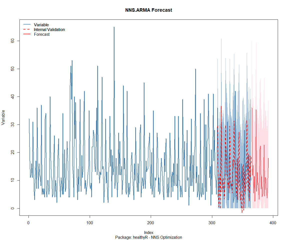
NNS Forecasting
This is something I have been wanting to try for a while. The NNS
package is a great package for forecasting time series data.
library(NNS)

data_list <- base_data |>
    select(package, value) |>
    group_split(package)

data_list |>
    imap(
        \(x, idx) {
            obj <- x
            x <- obj |> pull(value) |> tail(7*52)
            train_set_size <- length(x) - 56
            pkg <- obj |> pluck(1) |> unique()
#            sf <- NNS.seas(x, modulo = 7, plot = FALSE)$periods
            seas <- t(
                sapply(
                    1:25,
                    function(i) c(
                        i,
                        sqrt(
                            mean((
                                NNS.ARMA(x,
                                         h = 28,
                                         training.set = train_set_size,
                                         method = "lin",
                                         seasonal.factor = i,
                                         plot=FALSE
                                         ) - tail(x, 28)) ^ 2)))
                    )
                )
            colnames(seas) <- c("Period", "RMSE")
            sf <- seas[which.min(seas[, 2]), 1]

            cat(paste0("Package: ", pkg, "\n"))
            NNS.ARMA.optim(
                variable = x,
                h = 28,
                training.set = train_set_size,
                #seasonal.factor = seq(12, 60, 7),
                seasonal.factor = sf,
                pred.int = 0.95,
                plot = TRUE
            )
            title(
                sub = paste0("\n",
                             "Package: ", pkg, " - NNS Optimization")
            )
        }
    )
Package: healthyR
[1] "CURRNET METHOD: lin"
[1] "COPY LATEST PARAMETERS DIRECTLY FOR NNS.ARMA() IF ERROR:"
[1] "NNS.ARMA(... method =  'lin' , seasonal.factor =  c( 19 ) ...)"
[1] "CURRENT lin OBJECTIVE FUNCTION = 7.86960522115363"
[1] "BEST method = 'lin' PATH MEMBER = c( 19 )"
[1] "BEST lin OBJECTIVE FUNCTION = 7.86960522115363"
[1] "CURRNET METHOD: nonlin"
[1] "COPY LATEST PARAMETERS DIRECTLY FOR NNS.ARMA() IF ERROR:"
[1] "NNS.ARMA(... method =  'nonlin' , seasonal.factor =  c( 19 ) ...)"
[1] "CURRENT nonlin OBJECTIVE FUNCTION = 16.7893779546478"
[1] "BEST method = 'nonlin' PATH MEMBER = c( 19 )"
[1] "BEST nonlin OBJECTIVE FUNCTION = 16.7893779546478"
[1] "CURRNET METHOD: both"
[1] "COPY LATEST PARAMETERS DIRECTLY FOR NNS.ARMA() IF ERROR:"
[1] "NNS.ARMA(... method =  'both' , seasonal.factor =  c( 19 ) ...)"
[1] "CURRENT both OBJECTIVE FUNCTION = 12.1408061627669"
[1] "BEST method = 'both' PATH MEMBER = c( 19 )"
[1] "BEST both OBJECTIVE FUNCTION = 12.1408061627669"
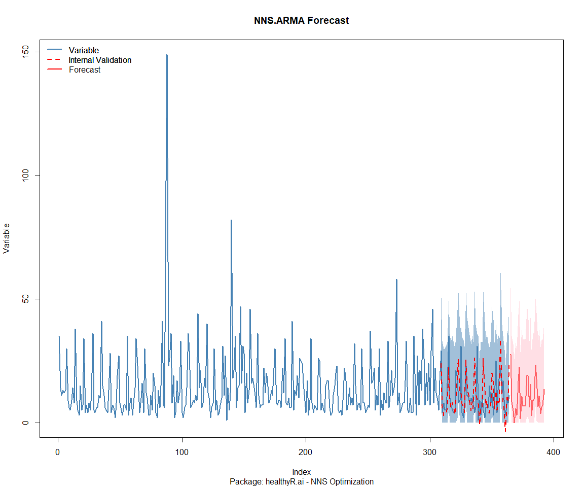
Package: healthyR.ai
[1] "CURRNET METHOD: lin"
[1] "COPY LATEST PARAMETERS DIRECTLY FOR NNS.ARMA() IF ERROR:"
[1] "NNS.ARMA(... method =  'lin' , seasonal.factor =  c( 5 ) ...)"
[1] "CURRENT lin OBJECTIVE FUNCTION = 14.2499959929283"
[1] "BEST method = 'lin' PATH MEMBER = c( 5 )"
[1] "BEST lin OBJECTIVE FUNCTION = 14.2499959929283"
[1] "CURRNET METHOD: nonlin"
[1] "COPY LATEST PARAMETERS DIRECTLY FOR NNS.ARMA() IF ERROR:"
[1] "NNS.ARMA(... method =  'nonlin' , seasonal.factor =  c( 5 ) ...)"
[1] "CURRENT nonlin OBJECTIVE FUNCTION = 8.17289805336758"
[1] "BEST method = 'nonlin' PATH MEMBER = c( 5 )"
[1] "BEST nonlin OBJECTIVE FUNCTION = 8.17289805336758"
[1] "CURRNET METHOD: both"
[1] "COPY LATEST PARAMETERS DIRECTLY FOR NNS.ARMA() IF ERROR:"
[1] "NNS.ARMA(... method =  'both' , seasonal.factor =  c( 5 ) ...)"
[1] "CURRENT both OBJECTIVE FUNCTION = 10.369821843814"
[1] "BEST method = 'both' PATH MEMBER = c( 5 )"
[1] "BEST both OBJECTIVE FUNCTION = 10.369821843814"
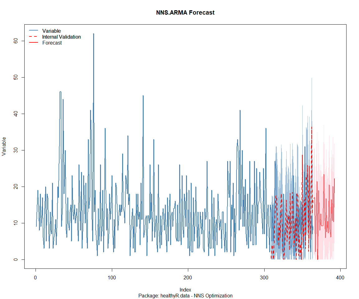
Package: healthyR.data
[1] "CURRNET METHOD: lin"
[1] "COPY LATEST PARAMETERS DIRECTLY FOR NNS.ARMA() IF ERROR:"
[1] "NNS.ARMA(... method =  'lin' , seasonal.factor =  c( 2 ) ...)"
[1] "CURRENT lin OBJECTIVE FUNCTION = 30.9318787023258"
[1] "BEST method = 'lin' PATH MEMBER = c( 2 )"
[1] "BEST lin OBJECTIVE FUNCTION = 30.9318787023258"
[1] "CURRNET METHOD: nonlin"
[1] "COPY LATEST PARAMETERS DIRECTLY FOR NNS.ARMA() IF ERROR:"
[1] "NNS.ARMA(... method =  'nonlin' , seasonal.factor =  c( 2 ) ...)"
[1] "CURRENT nonlin OBJECTIVE FUNCTION = 6.17661586488365"
[1] "BEST method = 'nonlin' PATH MEMBER = c( 2 )"
[1] "BEST nonlin OBJECTIVE FUNCTION = 6.17661586488365"
[1] "CURRNET METHOD: both"
[1] "COPY LATEST PARAMETERS DIRECTLY FOR NNS.ARMA() IF ERROR:"
[1] "NNS.ARMA(... method =  'both' , seasonal.factor =  c( 2 ) ...)"
[1] "CURRENT both OBJECTIVE FUNCTION = 4.14182683780808"
[1] "BEST method = 'both' PATH MEMBER = c( 2 )"
[1] "BEST both OBJECTIVE FUNCTION = 4.14182683780808"
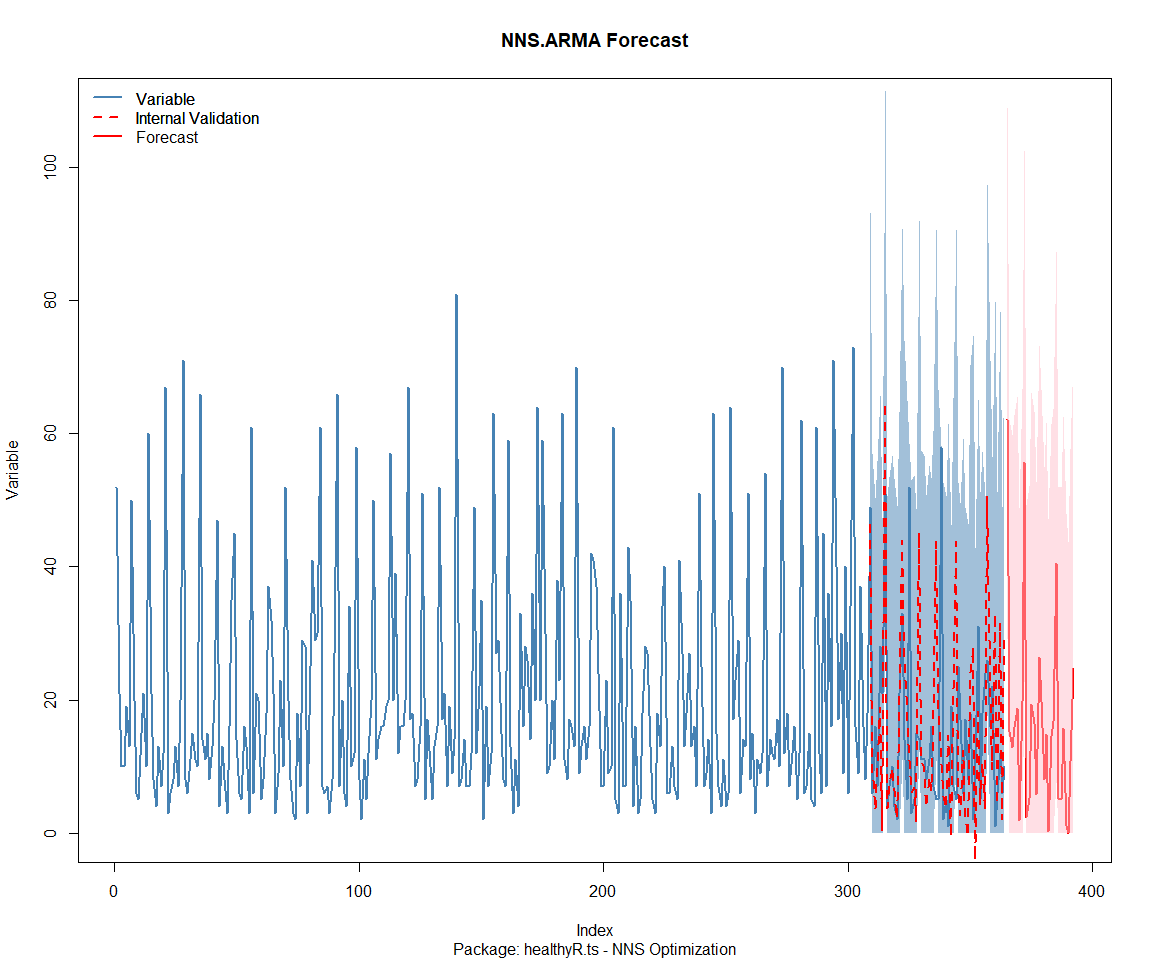
Package: healthyR.ts
[1] "CURRNET METHOD: lin"
[1] "COPY LATEST PARAMETERS DIRECTLY FOR NNS.ARMA() IF ERROR:"
[1] "NNS.ARMA(... method =  'lin' , seasonal.factor =  c( 10 ) ...)"
[1] "CURRENT lin OBJECTIVE FUNCTION = 25.404487133529"
[1] "BEST method = 'lin' PATH MEMBER = c( 10 )"
[1] "BEST lin OBJECTIVE FUNCTION = 25.404487133529"
[1] "CURRNET METHOD: nonlin"
[1] "COPY LATEST PARAMETERS DIRECTLY FOR NNS.ARMA() IF ERROR:"
[1] "NNS.ARMA(... method =  'nonlin' , seasonal.factor =  c( 10 ) ...)"
[1] "CURRENT nonlin OBJECTIVE FUNCTION = 14.6987963549132"
[1] "BEST method = 'nonlin' PATH MEMBER = c( 10 )"
[1] "BEST nonlin OBJECTIVE FUNCTION = 14.6987963549132"
[1] "CURRNET METHOD: both"
[1] "COPY LATEST PARAMETERS DIRECTLY FOR NNS.ARMA() IF ERROR:"
[1] "NNS.ARMA(... method =  'both' , seasonal.factor =  c( 10 ) ...)"
[1] "CURRENT both OBJECTIVE FUNCTION = 17.9837049019487"
[1] "BEST method = 'both' PATH MEMBER = c( 10 )"
[1] "BEST both OBJECTIVE FUNCTION = 17.9837049019487"
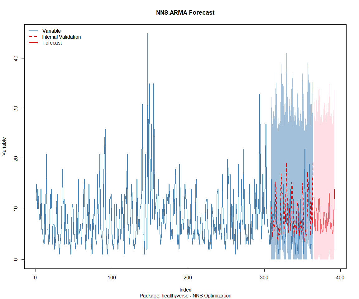
Package: healthyverse
[1] "CURRNET METHOD: lin"
[1] "COPY LATEST PARAMETERS DIRECTLY FOR NNS.ARMA() IF ERROR:"
[1] "NNS.ARMA(... method =  'lin' , seasonal.factor =  c( 11 ) ...)"
[1] "CURRENT lin OBJECTIVE FUNCTION = 7.74633073187101"
[1] "BEST method = 'lin' PATH MEMBER = c( 11 )"
[1] "BEST lin OBJECTIVE FUNCTION = 7.74633073187101"
[1] "CURRNET METHOD: nonlin"
[1] "COPY LATEST PARAMETERS DIRECTLY FOR NNS.ARMA() IF ERROR:"
[1] "NNS.ARMA(... method =  'nonlin' , seasonal.factor =  c( 11 ) ...)"
[1] "CURRENT nonlin OBJECTIVE FUNCTION = 4.67243603207911"
[1] "BEST method = 'nonlin' PATH MEMBER = c( 11 )"
[1] "BEST nonlin OBJECTIVE FUNCTION = 4.67243603207911"
[1] "CURRNET METHOD: both"
[1] "COPY LATEST PARAMETERS DIRECTLY FOR NNS.ARMA() IF ERROR:"
[1] "NNS.ARMA(... method =  'both' , seasonal.factor =  c( 11 ) ...)"
[1] "CURRENT both OBJECTIVE FUNCTION = 5.17396619116188"
[1] "BEST method = 'both' PATH MEMBER = c( 11 )"
[1] "BEST both OBJECTIVE FUNCTION = 5.17396619116188"
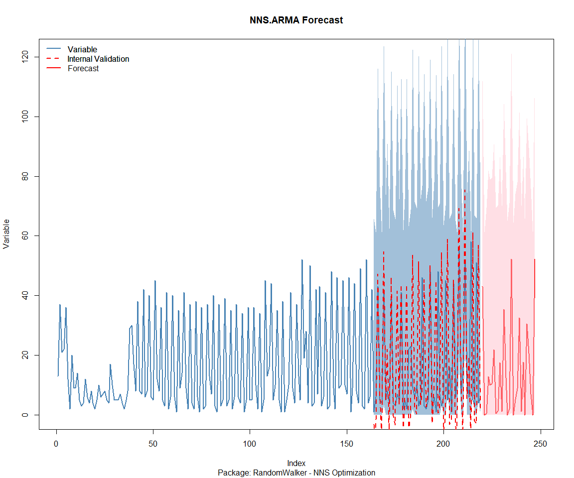
Package: RandomWalker
[1] "CURRNET METHOD: lin"
[1] "COPY LATEST PARAMETERS DIRECTLY FOR NNS.ARMA() IF ERROR:"
[1] "NNS.ARMA(... method =  'lin' , seasonal.factor =  c( 4 ) ...)"
[1] "CURRENT lin OBJECTIVE FUNCTION = 13.4063067542187"
[1] "BEST method = 'lin' PATH MEMBER = c( 4 )"
[1] "BEST lin OBJECTIVE FUNCTION = 13.4063067542187"
[1] "CURRNET METHOD: nonlin"
[1] "COPY LATEST PARAMETERS DIRECTLY FOR NNS.ARMA() IF ERROR:"
[1] "NNS.ARMA(... method =  'nonlin' , seasonal.factor =  c( 4 ) ...)"
[1] "CURRENT nonlin OBJECTIVE FUNCTION = 5.5676177002934"
[1] "BEST method = 'nonlin' PATH MEMBER = c( 4 )"
[1] "BEST nonlin OBJECTIVE FUNCTION = 5.5676177002934"
[1] "CURRNET METHOD: both"
[1] "COPY LATEST PARAMETERS DIRECTLY FOR NNS.ARMA() IF ERROR:"
[1] "NNS.ARMA(... method =  'both' , seasonal.factor =  c( 4 ) ...)"
[1] "CURRENT both OBJECTIVE FUNCTION = 5.73372891024602"
[1] "BEST method = 'both' PATH MEMBER = c( 4 )"
[1] "BEST both OBJECTIVE FUNCTION = 5.73372891024602"
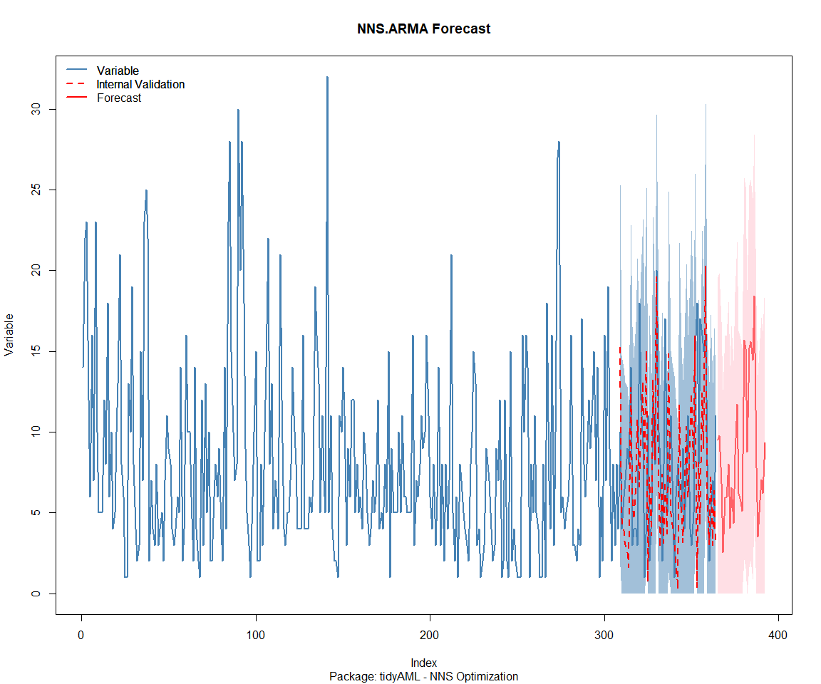
Package: tidyAML
[1] "CURRNET METHOD: lin"
[1] "COPY LATEST PARAMETERS DIRECTLY FOR NNS.ARMA() IF ERROR:"
[1] "NNS.ARMA(... method =  'lin' , seasonal.factor =  c( 4 ) ...)"
[1] "CURRENT lin OBJECTIVE FUNCTION = 6.08485316398437"
[1] "BEST method = 'lin' PATH MEMBER = c( 4 )"
[1] "BEST lin OBJECTIVE FUNCTION = 6.08485316398437"
[1] "CURRNET METHOD: nonlin"
[1] "COPY LATEST PARAMETERS DIRECTLY FOR NNS.ARMA() IF ERROR:"
[1] "NNS.ARMA(... method =  'nonlin' , seasonal.factor =  c( 4 ) ...)"
[1] "CURRENT nonlin OBJECTIVE FUNCTION = 8.54082307877222"
[1] "BEST method = 'nonlin' PATH MEMBER = c( 4 )"
[1] "BEST nonlin OBJECTIVE FUNCTION = 8.54082307877222"
[1] "CURRNET METHOD: both"
[1] "COPY LATEST PARAMETERS DIRECTLY FOR NNS.ARMA() IF ERROR:"
[1] "NNS.ARMA(... method =  'both' , seasonal.factor =  c( 4 ) ...)"
[1] "CURRENT both OBJECTIVE FUNCTION = 18.3159900519083"
[1] "BEST method = 'both' PATH MEMBER = c( 4 )"
[1] "BEST both OBJECTIVE FUNCTION = 18.3159900519083"
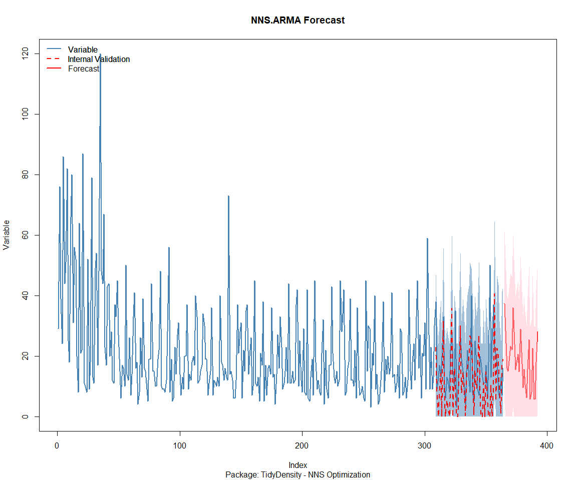
Package: TidyDensity
[1] "CURRNET METHOD: lin"
[1] "COPY LATEST PARAMETERS DIRECTLY FOR NNS.ARMA() IF ERROR:"
[1] "NNS.ARMA(... method =  'lin' , seasonal.factor =  c( 15 ) ...)"
[1] "CURRENT lin OBJECTIVE FUNCTION = 18.3453157168816"
[1] "BEST method = 'lin' PATH MEMBER = c( 15 )"
[1] "BEST lin OBJECTIVE FUNCTION = 18.3453157168816"
[1] "CURRNET METHOD: nonlin"
[1] "COPY LATEST PARAMETERS DIRECTLY FOR NNS.ARMA() IF ERROR:"
[1] "NNS.ARMA(... method =  'nonlin' , seasonal.factor =  c( 15 ) ...)"
[1] "CURRENT nonlin OBJECTIVE FUNCTION = 4.18386497460203"
[1] "BEST method = 'nonlin' PATH MEMBER = c( 15 )"
[1] "BEST nonlin OBJECTIVE FUNCTION = 4.18386497460203"
[1] "CURRNET METHOD: both"
[1] "COPY LATEST PARAMETERS DIRECTLY FOR NNS.ARMA() IF ERROR:"
[1] "NNS.ARMA(... method =  'both' , seasonal.factor =  c( 15 ) ...)"
[1] "CURRENT both OBJECTIVE FUNCTION = 4.63248908416527"
[1] "BEST method = 'both' PATH MEMBER = c( 15 )"
[1] "BEST both OBJECTIVE FUNCTION = 4.63248908416527"
[[1]]
NULL

[[2]]
NULL

[[3]]
NULL

[[4]]
NULL

[[5]]
NULL

[[6]]
NULL

[[7]]
NULL

[[8]]
NULL
Pre-Processing
Now we are going to do some basic pre-processing.
data_padded_tbl <- base_data %>%
  pad_by_time(
    .date_var  = date,
    .pad_value = 0
  )

# Get log interval and standardization parameters
log_params  <- liv(data_padded_tbl$value, limit_lower = 0, offset = 1, silent = TRUE)
limit_lower <- log_params$limit_lower
limit_upper <- log_params$limit_upper
offset      <- log_params$offset

data_liv_tbl <- data_padded_tbl %>%
  # Get log interval transform
  mutate(value_trans = liv(value, limit_lower = 0, offset = 1, silent = TRUE)$log_scaled)

# Get Standardization Params
std_params <- standard_vec(data_liv_tbl$value_trans, silent = TRUE)
std_mean   <- std_params$mean
std_sd     <- std_params$sd

data_transformed_tbl <- data_liv_tbl %>%
  group_by(package) %>%
  # get standardization
  mutate(value_trans = standard_vec(value_trans, silent = TRUE)$standard_scaled) %>%
  tk_augment_fourier(
    .date_var = date,
    .periods  = c(7, 14, 30, 90, 180),
    .K        = 2
  ) %>%
  tk_augment_timeseries_signature(
    .date_var = date
  ) %>%
  ungroup() %>%
  select(-c(value, -year.iso))
Since this is panel data we can follow one of two different modeling strategies. We can search for a global model in the panel data or we can use nested forecasting finding the best model for each of the time series. Since we only have 5 panels, we will use nested forecasting.
To do this we will use the nest_timeseries and
split_nested_timeseries functions to create a nested tibble.
horizon <- 4*7

nested_data_tbl <- data_transformed_tbl %>%

    # 0. Filter out column where package is NA
    filter(!is.na(package)) %>%

    # 1. Extending: We'll predict n days into the future.
    extend_timeseries(
        .id_var        = package,
        .date_var      = date,
        .length_future = horizon
    ) %>%

    # 2. Nesting: We'll group by id, and create a future dataset
    #    that forecasts n days of extended data and
    #    an actual dataset that contains n*2 days
    nest_timeseries(
        .id_var        = package,
        .length_future = horizon
        #.length_actual = horizon*2
    ) %>%

   # 3. Splitting: We'll take the actual data and create splits
   #    for accuracy and confidence interval estimation of n das (test)
   #    and the rest is training data
    split_nested_timeseries(
        .length_test = horizon
    )

nested_data_tbl
# A tibble: 8 × 4
  package       .actual_data          .future_data       .splits
  <fct>         <list>                <list>             <list>
1 healthyR.data <tibble [2,011 × 50]> <tibble [28 × 50]> <split [1983|28]>
2 healthyR      <tibble [2,004 × 50]> <tibble [28 × 50]> <split [1976|28]>
3 healthyR.ts   <tibble [1,940 × 50]> <tibble [28 × 50]> <split [1912|28]>
4 healthyverse  <tibble [1,859 × 50]> <tibble [28 × 50]> <split [1831|28]>
5 healthyR.ai   <tibble [1,746 × 50]> <tibble [28 × 50]> <split [1718|28]>
6 TidyDensity   <tibble [1,598 × 50]> <tibble [28 × 50]> <split [1570|28]>
7 tidyAML       <tibble [1,203 × 50]> <tibble [28 × 50]> <split [1175|28]>
8 RandomWalker  <tibble [626 × 50]>   <tibble [28 × 50]> <split [598|28]>
Now it is time to make some recipes and models using the modeltime workflow.
Modeltime Workflow
Recipe Object
recipe_base <- recipe(
  value_trans ~ .
  , data = extract_nested_test_split(nested_data_tbl)
  )

recipe_base

recipe_date <- recipe(
  value_trans ~ date
  , data = extract_nested_test_split(nested_data_tbl)
  )
Models
# Models ------------------------------------------------------------------

# Auto ARIMA --------------------------------------------------------------

model_spec_arima_no_boost <- arima_reg() %>%
  set_engine(engine = "auto_arima")

wflw_auto_arima <- workflow() %>%
  add_recipe(recipe = recipe_date) %>%
  add_model(model_spec_arima_no_boost)

# NNETAR ------------------------------------------------------------------

model_spec_nnetar <- nnetar_reg(
  mode              = "regression"
  , seasonal_period = "auto"
) %>%
  set_engine("nnetar")

wflw_nnetar <- workflow() %>%
  add_recipe(recipe = recipe_base) %>%
  add_model(model_spec_nnetar)

# TSLM --------------------------------------------------------------------

model_spec_lm <- linear_reg() %>%
  set_engine("lm")

wflw_lm <- workflow() %>%
  add_recipe(recipe = recipe_base) %>%
  add_model(model_spec_lm)

# MARS --------------------------------------------------------------------

model_spec_mars <- mars(mode = "regression") %>%
  set_engine("earth")

wflw_mars <- workflow() %>%
  add_recipe(recipe = recipe_date) %>%
  add_model(model_spec_mars)
Nested Modeltime Tables
nested_modeltime_tbl <- modeltime_nested_fit(
  # Nested Data
  nested_data = nested_data_tbl,
   control = control_nested_fit(
     verbose = TRUE,
     allow_par = FALSE
   ),
  # Add workflows
  wflw_auto_arima,
  wflw_lm,
  wflw_mars,
  wflw_nnetar
)
nested_modeltime_tbl <- nested_modeltime_tbl[!is.na(nested_modeltime_tbl$package),]
Model Accuracy
nested_modeltime_tbl %>%
  extract_nested_test_accuracy() %>%
  filter(!is.na(package)) %>%
  knitr::kable()
| package | .model_id | .model_desc | .type | mae | mape | mase | smape | rmse | rsq |
|---|---|---|---|---|---|---|---|---|---|
| healthyR.data | 1 | ARIMA | Test | 0.6419525 | 149.20484 | 0.8814435 | 179.04018 | 0.7569412 | 0.0137647 |
| healthyR.data | 2 | LM | Test | 0.7117758 | 308.40272 | 0.9773155 | 149.10132 | 0.8320489 | 0.1977230 |
| healthyR.data | 3 | EARTH | Test | 0.6056508 | 131.83636 | 0.8315988 | 167.43438 | 0.7316991 | 0.1786895 |
| healthyR.data | 4 | NNAR | Test | 0.6660164 | 266.74546 | 0.9144848 | 145.28567 | 0.7978403 | 0.2015959 |
| healthyR | 1 | ARIMA | Test | 0.8284023 | 233.75462 | 0.7282521 | 141.14026 | 1.0249320 | 0.0079302 |
| healthyR | 2 | LM | Test | 0.8509996 | 339.66948 | 0.7481175 | 131.57622 | 0.9830068 | 0.1642929 |
| healthyR | 3 | EARTH | Test | 0.8213522 | 159.02148 | 0.7220543 | 155.16373 | 1.0264196 | 0.1641755 |
| healthyR | 4 | NNAR | Test | 0.8317844 | 232.72519 | 0.7312252 | 137.25593 | 0.9673483 | 0.1848346 |
| healthyR.ts | 1 | ARIMA | Test | 0.8064509 | 1005.71408 | 0.6884423 | 174.48921 | 1.0658929 | 0.0033104 |
| healthyR.ts | 2 | LM | Test | 0.8092933 | 5807.43279 | 0.6908687 | 137.28316 | 1.0309414 | 0.0599232 |
| healthyR.ts | 3 | EARTH | Test | 0.7894332 | 503.75987 | 0.6739148 | 188.59284 | 1.0632205 | 0.0558901 |
| healthyR.ts | 4 | NNAR | Test | 0.8607467 | 5181.98601 | 0.7347929 | 144.42459 | 1.0630839 | 0.0369219 |
| healthyverse | 1 | ARIMA | Test | 0.6076595 | 67.69716 | 0.9796602 | 48.50801 | 0.7049081 | 0.0028713 |
| healthyverse | 2 | LM | Test | 0.7828216 | 53.63642 | 1.2620542 | 67.85047 | 0.9288244 | 0.0730920 |
| healthyverse | 3 | EARTH | Test | 0.5096417 | 72.64375 | 0.8216373 | 39.37889 | 0.6547186 | 0.0811721 |
| healthyverse | 4 | NNAR | Test | 0.8437787 | 56.04175 | 1.3603284 | 71.85020 | 0.9793257 | 0.0219135 |
| healthyR.ai | 1 | ARIMA | Test | 0.7627802 | 125.18473 | 0.7115371 | 124.48028 | 0.9655930 | 0.0262763 |
| healthyR.ai | 2 | LM | Test | 0.7410388 | 196.06956 | 0.6912562 | 107.10194 | 0.9454672 | 0.1229999 |
| healthyR.ai | 3 | EARTH | Test | 0.8289453 | 101.74403 | 0.7732573 | 186.95702 | 0.9958711 | 0.1139203 |
| healthyR.ai | 4 | NNAR | Test | 0.6984244 | 162.09065 | 0.6515046 | 112.04554 | 0.8939179 | 0.1922032 |
| TidyDensity | 1 | ARIMA | Test | 0.8713763 | 105.44142 | 0.7149494 | 152.60132 | 1.0645959 | 0.0269340 |
| TidyDensity | 2 | LM | Test | 0.8582987 | 129.12061 | 0.7042195 | 132.21143 | 1.0401625 | 0.0458691 |
| TidyDensity | 3 | EARTH | Test | 0.8713879 | 131.98706 | 0.7149589 | 132.19588 | 1.0340778 | 0.0271018 |
| TidyDensity | 4 | NNAR | Test | 0.8118321 | 130.49282 | 0.6660944 | 131.78774 | 0.9778372 | 0.1845398 |
| tidyAML | 1 | ARIMA | Test | 0.6971148 | 117.75439 | 0.7160331 | 165.31279 | 0.8454759 | 0.0105182 |
| tidyAML | 2 | LM | Test | 0.9083520 | 243.56621 | 0.9330029 | 142.27546 | 1.1007620 | 0.0223254 |
| tidyAML | 3 | EARTH | Test | 0.7425821 | 161.80939 | 0.7627343 | 151.32944 | 0.8729054 | 0.1316865 |
| tidyAML | 4 | NNAR | Test | 0.9176139 | 226.22095 | 0.9425162 | 159.24605 | 1.0998257 | 0.0572586 |
| RandomWalker | 1 | ARIMA | Test | 0.9121344 | 122.28054 | 0.7261153 | 160.32625 | 1.0818559 | 0.0022176 |
| RandomWalker | 2 | LM | Test | 0.8386647 | 94.23770 | 0.6676289 | 158.79904 | 1.0275259 | 0.0015594 |
| RandomWalker | 3 | EARTH | Test | 0.8678233 | 99.91551 | 0.6908409 | 190.60973 | 1.0195793 | 0.0013927 |
| RandomWalker | 4 | NNAR | Test | 1.0232515 | 141.96029 | 0.8145713 | 173.96347 | 1.1841113 | 0.1449539 |
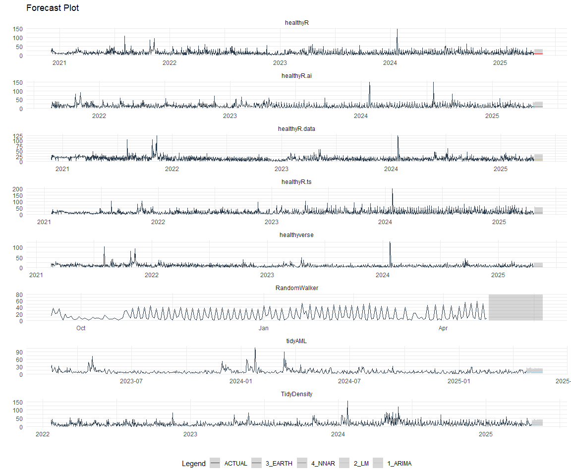
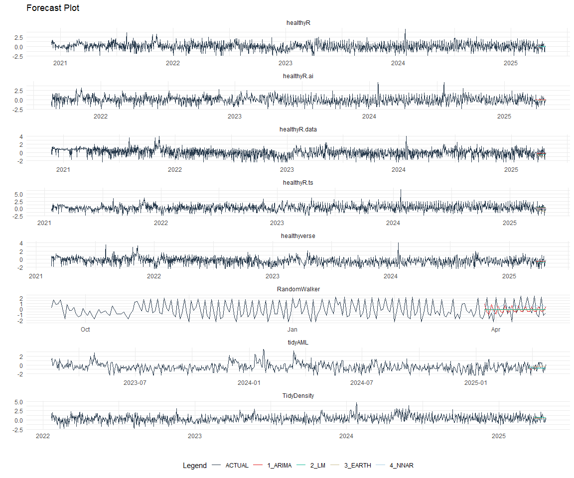
Plot Models
nested_modeltime_tbl %>%
  extract_nested_test_forecast() %>%
  group_by(package) %>%
  filter_by_time(.date_var = .index, .start_date = max(.index) - 60) %>%
  ungroup() %>%
  plot_modeltime_forecast(
    .interactive = FALSE,
    .conf_interval_show  = FALSE,
    .facet_scales = "free"
  ) +
  theme_minimal() +
  facet_wrap(~ package, nrow = 3) +
  theme(legend.position = "bottom")
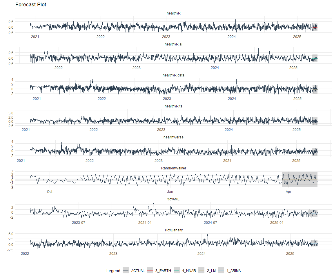
Best Model
best_nested_modeltime_tbl <- nested_modeltime_tbl %>%
  modeltime_nested_select_best(
    metric = "rmse",
    minimize = TRUE,
    filter_test_forecasts = TRUE
  )

best_nested_modeltime_tbl %>%
  extract_nested_best_model_report()
# Nested Modeltime Table


# A tibble: 8 × 10
  package     .model_id .model_desc .type   mae   mape  mase smape  rmse     rsq
  <fct>           <int> <chr>       <chr> <dbl>  <dbl> <dbl> <dbl> <dbl>   <dbl>
1 healthyR.d…         3 EARTH       Test  0.606  132.  0.832 167.  0.732 0.179
2 healthyR            4 NNAR        Test  0.832  233.  0.731 137.  0.967 0.185
3 healthyR.ts         2 LM          Test  0.809 5807.  0.691 137.  1.03  0.0599
4 healthyver…         3 EARTH       Test  0.510   72.6 0.822  39.4 0.655 0.0812
5 healthyR.ai         4 NNAR        Test  0.698  162.  0.652 112.  0.894 0.192
6 TidyDensity         4 NNAR        Test  0.812  130.  0.666 132.  0.978 0.185
7 tidyAML             1 ARIMA       Test  0.697  118.  0.716 165.  0.845 0.0105
8 RandomWalk…         3 EARTH       Test  0.868   99.9 0.691 191.  1.02  0.00139
best_nested_modeltime_tbl %>%
  extract_nested_test_forecast() %>%
  #filter(!is.na(.model_id)) %>%
  group_by(package) %>%
  filter_by_time(.date_var = .index, .start_date = max(.index) - 60) %>%
  ungroup() %>%
  plot_modeltime_forecast(
    .interactive = FALSE,
    .conf_interval_alpha = 0.2,
    .facet_scales = "free"
  ) +
  facet_wrap(~ package, nrow = 3) +
  theme_minimal() +
  theme(legend.position = "bottom")
Refitting and Future Forecast
Now that we have the best models, we can make our future forecasts.
nested_modeltime_refit_tbl <- best_nested_modeltime_tbl %>%
    modeltime_nested_refit(
        control = control_nested_refit(verbose = TRUE)
    )
nested_modeltime_refit_tbl
# Nested Modeltime Table


# A tibble: 8 × 5
  package       .actual_data .future_data .splits           .modeltime_tables
  <fct>         <list>       <list>       <list>            <list>
1 healthyR.data <tibble>     <tibble>     <split [1983|28]> <mdl_tm_t [1 × 5]>
2 healthyR      <tibble>     <tibble>     <split [1976|28]> <mdl_tm_t [1 × 5]>
3 healthyR.ts   <tibble>     <tibble>     <split [1912|28]> <mdl_tm_t [1 × 5]>
4 healthyverse  <tibble>     <tibble>     <split [1831|28]> <mdl_tm_t [1 × 5]>
5 healthyR.ai   <tibble>     <tibble>     <split [1718|28]> <mdl_tm_t [1 × 5]>
6 TidyDensity   <tibble>     <tibble>     <split [1570|28]> <mdl_tm_t [1 × 5]>
7 tidyAML       <tibble>     <tibble>     <split [1175|28]> <mdl_tm_t [1 × 5]>
8 RandomWalker  <tibble>     <tibble>     <split [598|28]>  <mdl_tm_t [1 × 5]>
nested_modeltime_refit_tbl %>%
  extract_nested_future_forecast() %>%
  group_by(package) %>%
  mutate(across(.value:.conf_hi, .fns = ~ standard_inv_vec(
    x    = .,
    mean = std_mean,
    sd   = std_sd
  )$standard_inverse_value)) %>%
  mutate(across(.value:.conf_hi, .fns = ~ liiv(
    x = .,
    limit_lower = limit_lower,
    limit_upper = limit_upper,
    offset      = offset
  )$rescaled_v)) %>%
  filter_by_time(.date_var = .index, .start_date = max(.index) - 60) %>%
  ungroup() %>%
  plot_modeltime_forecast(
    .interactive = FALSE,
    .conf_interval_alpha = 0.2,
    .facet_scales = "free"
  ) +
  facet_wrap(~ package, nrow = 3) +
  theme_minimal() +
  theme(legend.position = "bottom")