Introduction

Are you tired of dealing with irregularly spaced data points that just don’t seem to fit together? Do you find yourself struggling to interpolate or smooth your data for better analysis? Look no further! In this blog post, we’ll dive deep into the powerful world of data approximation using R’s approx() function. Buckle up, because by the end of this journey, you’ll have a new tool in your R toolkit that can help you tame even the wildest datasets.

Understanding the Syntax

Before we jump into examples, let’s get a grasp of the approx() function’s syntax. The function is primarily used to perform linear interpolation on a dataset. The basic syntax is as follows:

approx(x, y, xout, method = "linear", rule = 2, f = 0, ties = mean)

x: The input vector of x-coordinates (independent variable).
y: The input vector of y-coordinates (dependent variable).
xout: The vector of x-coordinates where you want to approximate the corresponding y-values.
method: The interpolation method, typically “linear” for linear interpolation.
rule: A numerical value specifying how to handle points outside the range of x. Default is 2, which means to extrapolate.
f: A smoothing parameter. Set it between 0 and 1 to get a smoother approximation.
ties: How to handle tied values. Default is to take the mean.

Examples

Example 1: Basic Linear Interpolation

Suppose you have a dataset of temperature measurements at irregular intervals and you want to estimate the temperature at a specific time. Here’s how approx() can help:

# Sample data
time <- c(0, 2, 5, 8, 10)
temperature <- c(20, 25, 30, 28, 22)

# Time point to estimate temperature
time_estimate <- 6

# Using approx() for linear interpolation
approximated_temp <- approx(time, temperature, xout = time_estimate)$y

cat("Estimated temperature at time", time_estimate, "is", approximated_temp, "°C\n")

Estimated temperature at time 6 is 29.33333 °C

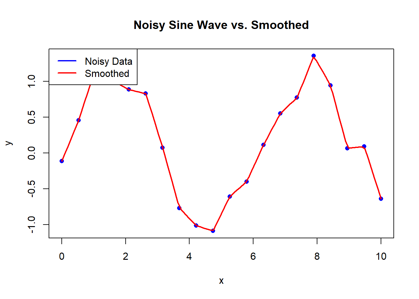
Example 2: Smoothing Out Noisy Data

Noisy data can be a nightmare for analysis. Let’s say you have a dataset with some irregularly spaced noisy sine wave points, and you want to create a smoother curve:

# Generating noisy sine wave data
set.seed(123)
x <- seq(0, 10, length.out = 20)
y <- sin(x) + rnorm(length(x), mean = 0, sd = 0.2)

# Smoothing out the curve
smoothed <- approx(x, y, xout = seq(0, 10, length.out = 100), f = 0.5)$y

# Plotting the original and smoothed data
plot(x, y, main = "Noisy Sine Wave vs. Smoothed", type = "p", col = "blue", pch = 16)
lines(seq(0, 10, length.out = 100), smoothed, col = "red", lwd = 2)
legend("topleft", legend = c("Noisy Data", "Smoothed"), col = c("blue", "red"), lwd = 2)

Get Hands-On with Your Data!

Are you excited yet? It’s time to get your hands dirty with the approx() function. Grab your own dataset, whether it’s irregularly spaced time-series data, scattered experimental measurements, or anything else that needs interpolation or smoothing. The examples provided should give you a solid foundation to start with. Remember, practice makes perfect!

In conclusion, R’s approx() function is a versatile tool for approximating data points, smoothing out noise, and filling in gaps in your datasets. By understanding its syntax and trying out various examples, you’ll be well-equipped to handle a wide range of data approximation tasks. So, what are you waiting for? Go ahead and embark on your journey to mastering the art of data approximation with R!