Introduction

When it comes to analyzing multivariate data, Principal Component Analysis (PCA) is a powerful technique that can help us uncover hidden patterns, reduce dimensionality, and gain valuable insights. One of the most informative ways to visualize the results of a PCA is by creating a biplot, and in this blog post, we’ll dive into how to do this using the biplot() function in R. To make it more practical, we’ll use the USArrests dataset to demonstrate the process step by step.

What is a Biplot?

Before we get into the details, let’s briefly discuss what a biplot is. A biplot is a graphical representation of a PCA that combines both the scores and loadings into a single plot. The scores represent the data points projected onto the principal components, while the loadings indicate the contribution of each original variable to the principal components. By plotting both, we can see how variables and data points relate to each other in a single chart, making it easier to interpret and analyze the PCA results.

Getting Started

First, if you haven’t already, load the necessary R packages. You’ll need the stats package for PCA and the biplot visualization.

# Load required packages
library(stats)

Performing PCA

Next, let’s perform PCA on the USArrests dataset using the prcomp() function, which is an R function for PCA. We’ll store the PCA results in a variable called pca_result.

# Perform PCA
pca_result <- prcomp(USArrests, scale = TRUE)

In the code above, we’ve scaled the data (scale = TRUE) to ensure that variables with different scales don’t dominate the PCA.

Creating the Biplot

Now comes the exciting part—creating the biplot! We’ll use the biplot() function to achieve this.

# Create a biplot
biplot(pca_result)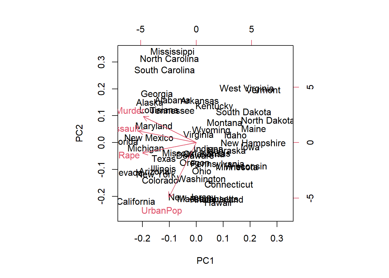

When you run the biplot() function with your PCA results, R will generate a biplot that combines both the scores and loadings. You’ll see arrows representing the original variables’ contributions to each principal component, and you’ll also see how the data points project onto the components.

Interpreting the Biplot

Let’s break down what you’ll see in the biplot:

Data Points: Each point represents a US state in our case, and its position in the biplot indicates how it relates to the principal components.
Arrows: The arrows represent the original variables (in this case, the crime statistics) and show how they contribute to the principal components. Longer arrows indicate stronger contributions.
Principal Components: The biplot will typically show the first two principal components. These components capture the most variation in the data.

What Insights Can You Gain?

By examining the biplot, you can draw several conclusions:

Clustering: States close to each other on the plot share similar crime profiles.
Variable Relationships: Variables close to each other on the plot are positively correlated, while those far apart are negatively correlated.
Outliers: States far from the center may be outliers in terms of their crime statistics.

Try It Yourself!

Now that you’ve seen how to create a biplot for PCA using the USArrests dataset, I encourage you to try it with your own data. PCA and biplots are powerful tools for dimensionality reduction and data exploration. They can help you uncover patterns, relationships, and outliers in your data, making it easier to make informed decisions in various fields, from biology to finance.

In this tutorial, we’ve barely scratched the surface of what you can do with PCA and biplots. Dive deeper, explore different datasets, and use this knowledge to gain valuable insights into your own multivariate data. Happy analyzing!