Introduction

Support Vector Machines (SVM) are a powerful tool in the world of machine learning and classification. They excel in finding the optimal decision boundary between different classes of data. However, understanding and visualizing these decision boundaries can be a bit tricky. In this blog post, we’ll explore how to plot an SVM object using the e1071 library in R, making it easier to grasp the magic happening under the hood.

What is e1071?

e1071 is an R package that provides tools for performing support vector machine (SVM) classification and regression. It’s widely used in the R community for its simplicity and efficiency. In this post, we’ll focus on SVM classification.

Setting Up

Before we dive into plotting, you’ll need to install and load the e1071 package if you haven’t already (I already have it so I won’t re-install it). You can do this using the following commands:

# Install e1071 (if not already installed)
# install.packages("e1071")

# Load the library
library(e1071)

Creating an Example SVM

Let’s start with a simple example to illustrate how to plot the decision boundary of an SVM. We’ll use a toy dataset with two classes: red dots and blue squares. Our goal is to create an SVM that separates these two classes.

# Create a toy dataset
set.seed(123)
data <- data.frame(
  x1 = rnorm(50, mean = 2),
  x2 = rnorm(50, mean = 2),
  label = c(rep("Red", 25), rep("Blue", 25)) |> as.factor()
)

# Train an SVM
svm_model <- svm(label ~ ., data = data, kernel = "linear")

In this example, we generated 50 data points with two features (x1 and x2) and two classes (Red and Blue). We then trained a linear SVM using the svm function from the e1071 package.

Plotting the Decision Boundary

Now comes the exciting part – plotting the decision boundary! We’ll use a combination of functions to achieve this. First, we’ll create a grid of points that cover the entire range of our data. Then, we’ll use the SVM model to predict the class labels for these points, effectively creating a decision boundary.

# Create a grid of points for prediction
x1_grid <- seq(min(data$x1), max(data$x1), length.out = 100)
x2_grid <- seq(min(data$x2), max(data$x2), length.out = 100)
grid <- expand.grid(x1 = x1_grid, x2 = x2_grid)

# Predict class labels for the grid
predicted_labels <- predict(svm_model, newdata = grid)

# Plot the decision boundary
plot(data$x1, data$x2, col = factor(data$label), pch = 19, main = "SVM Decision Boundary")
points(grid$x1, grid$x2, col = factor(predicted_labels), pch = ".", cex = 1.5)
legend("topright", legend = levels(data$label), col = c("blue", "red"), pch = 19)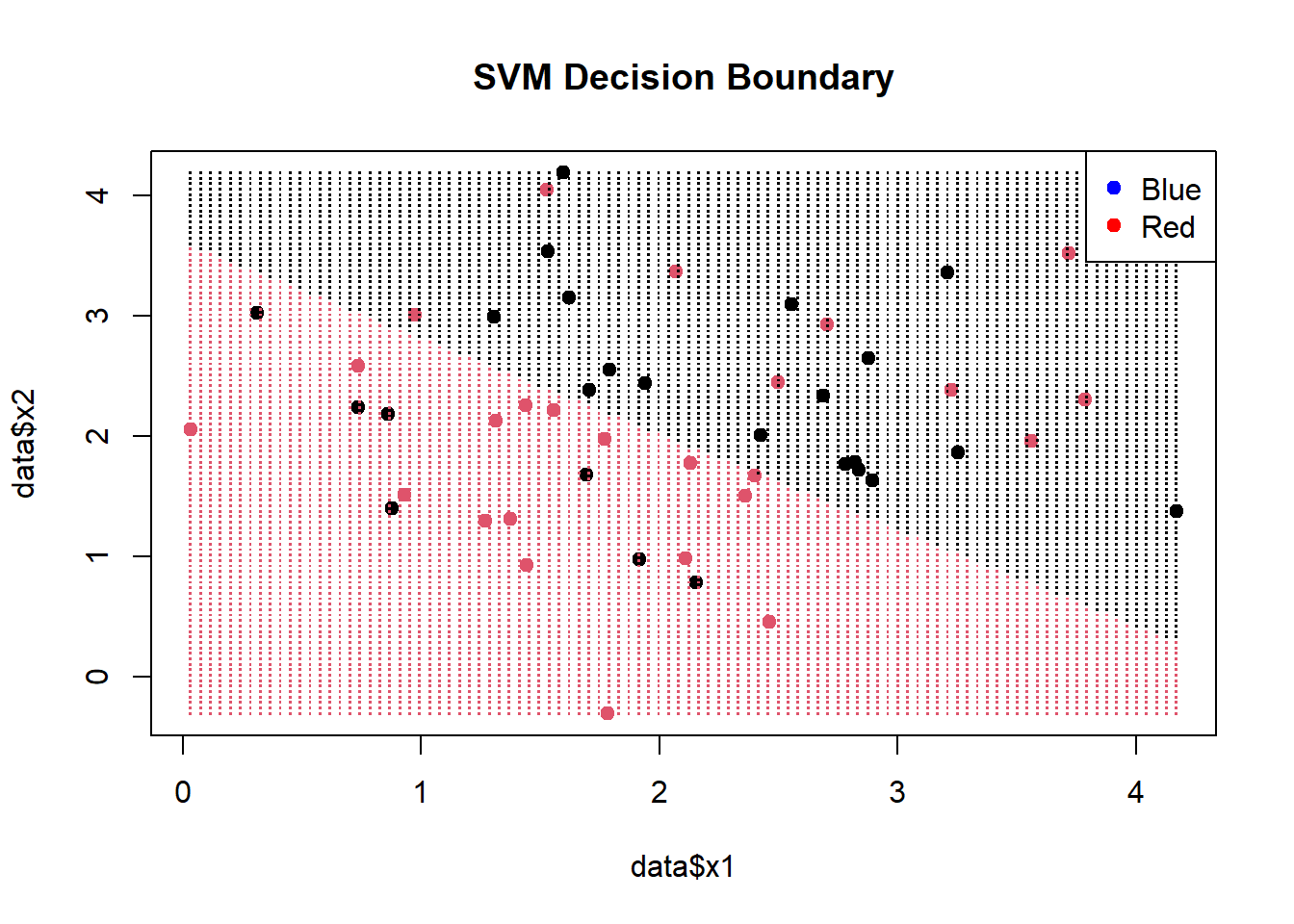

In this code, we first create a grid of points covering the range of our data using expand.grid. Then, we predict the class labels for these points using our trained SVM model and store them in predicted_labels. Finally, we plot the original data points with colors representing their true labels and overlay the decision boundary using the predicted labels.

Interpreting the Plot

The resulting plot will display your data points with red dots and blue squares, representing the true class labels. The decision boundary will be shown as a mix of red and blue points, indicating where the SVM has classified the data. The legend on the top-right helps you distinguish between the two classes.

We can also more simply plot out the model, see below:

plot(svm_model, data = data)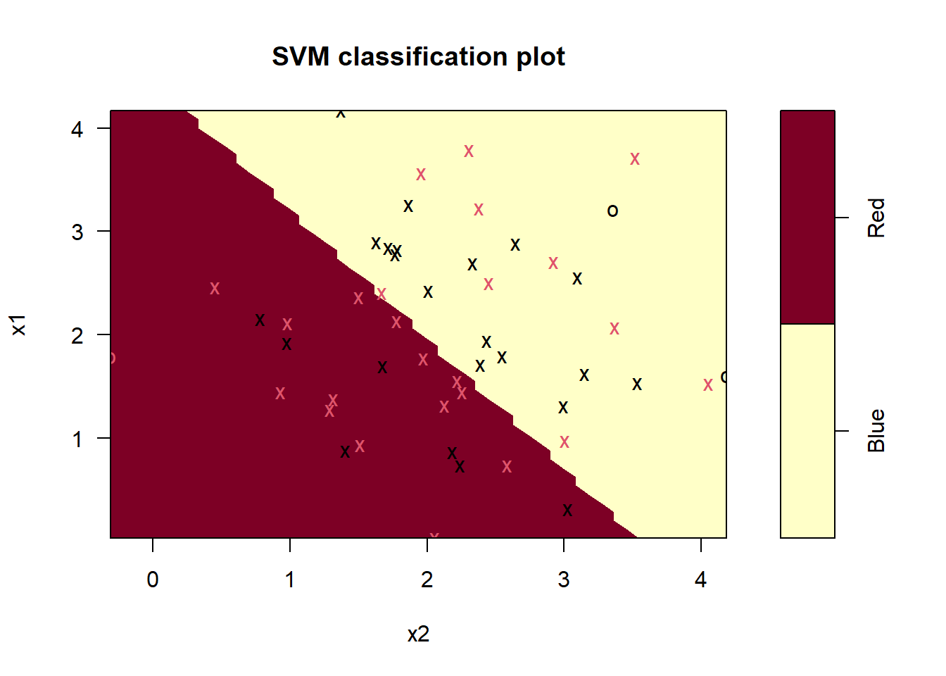

# Change the colors
plot(svm_model, data = data, color.palette = heat.colors)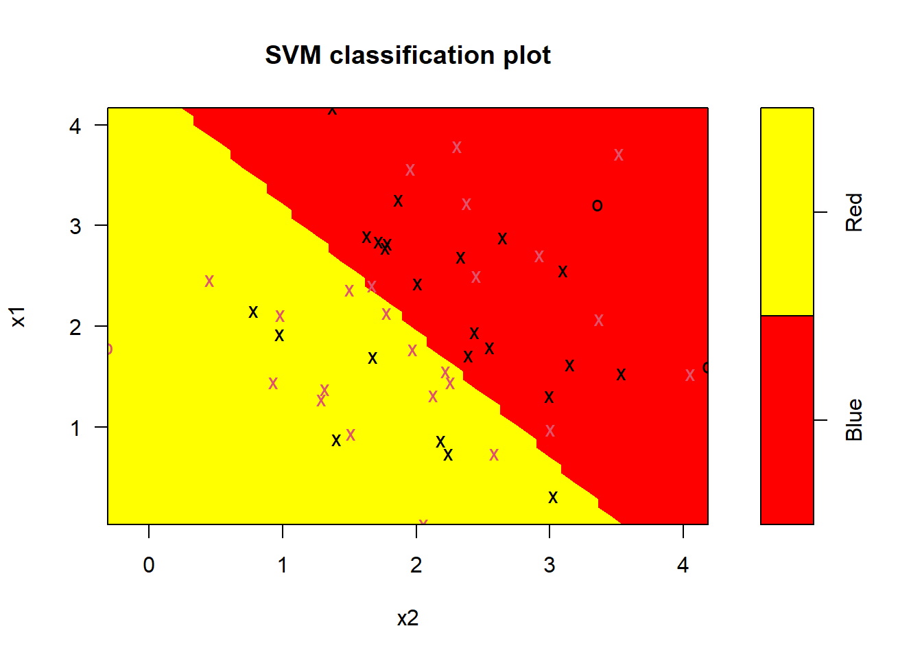

Try It Yourself!

Now that you’ve seen how to plot an SVM decision boundary using the e1071 package, I encourage you to try it with your own datasets and experiment with different kernels (e.g., radial or polynomial) to see how the decision boundary changes.

SVMs are a versatile tool for classification tasks, and visualizing their decision boundaries can provide valuable insights into your data and model. Happy plotting!