library(MASS)

# Simulate 100 observations from a bivariate normal distribution
set.seed(123) # Set a seed for reproducibility
bvnData <- mvrnorm(
  n = 100,
  mu = c(10, 20),
  Sigma = matrix(c(5, 3, 3, 6),
                 ncol = 2)
)Introduction
Welcome to the fascinating world of bivariate normal distributions! In this blog post, we’ll embark on a journey to understand, simulate, and visualize these distributions using the powerful R programming language. Whether you’re a seasoned R expert or a curious beginner, this guide will equip you with the necessary tools to explore this intriguing aspect of probability theory.
Understanding Bivariate Normal Distributions
Imagine two variables, like height and weight, that exhibit a joint distribution. The bivariate normal distribution captures the relationship between these variables, describing how their values tend to cluster around certain means and how they vary together. It’s like a two-dimensional bell curve, where the peak represents the most likely combination of values for both variables.
Simulating a Bivariate Normal Distribution
Now, let’s bring this distribution to life using R. The MASS package provides the mvrnorm() function, which generates random samples from a multivariate normal distribution. We’ll use this function to simulate a bivariate normal distribution with mean vector [10, 20] and covariance matrix [[5, 3], [3, 6]]. These parameters determine the center and shape of the distribution.
Visualizing the Bivariate Normal Distribution
To truly appreciate the beauty of the bivariate normal distribution, let’s visualize it using the plot() and density() functions
library(mnormt)

x <- bvnData[,1] |> sort()
y <- bvnData[,2] |> sort()
mu <- c(10, 20)
sigma <- matrix(c(5, 3, 3, 6),
                 ncol = 2)
f <- function(x, y) dmnorm(cbind(x, y), mu, sigma)
z <- outer(x,y,f)
contour(x,y,z)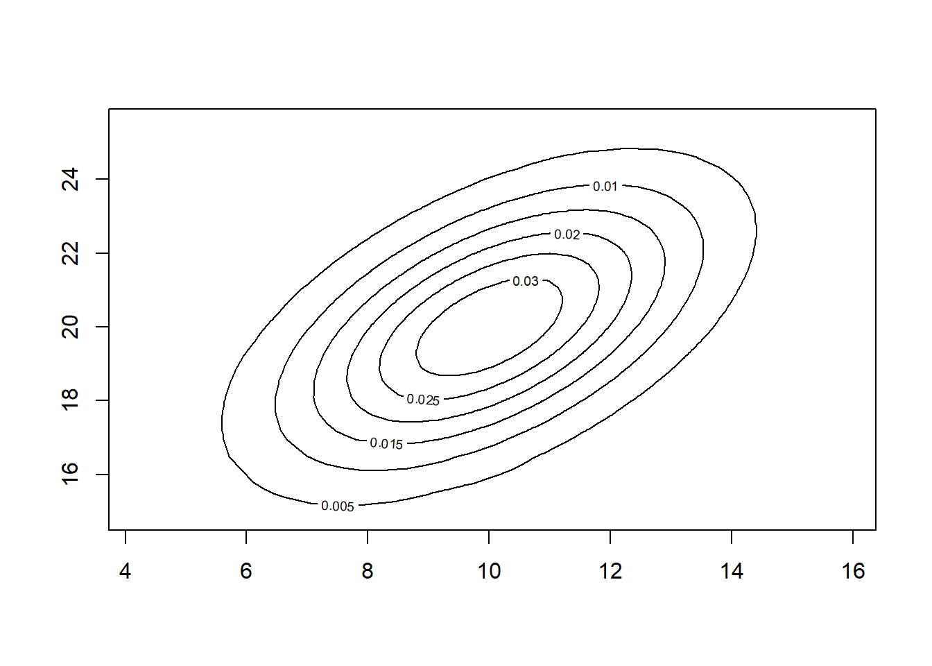
# Create a density plot of the simulated data
plot(density(bvnData))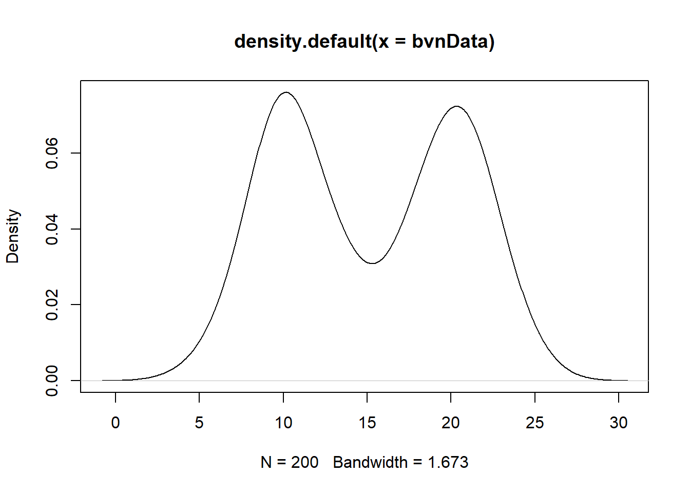
This plot should reveal an elliptical shape, with the highest density concentrated around the mean values. The contours represent the regions of equal probability.
Try It On Your Own!
Now, it’s your turn to experiment! Change the mean vector, covariance matrix, and sample size to see how they affect the shape and spread of the distribution. Play with different visualization options to explore different perspectives of the data.
Remember, R is a vast and ever-evolving language, so there’s always more to learn. Keep exploring, asking questions, and seeking out new challenges to become a master R programmer.