Introduction

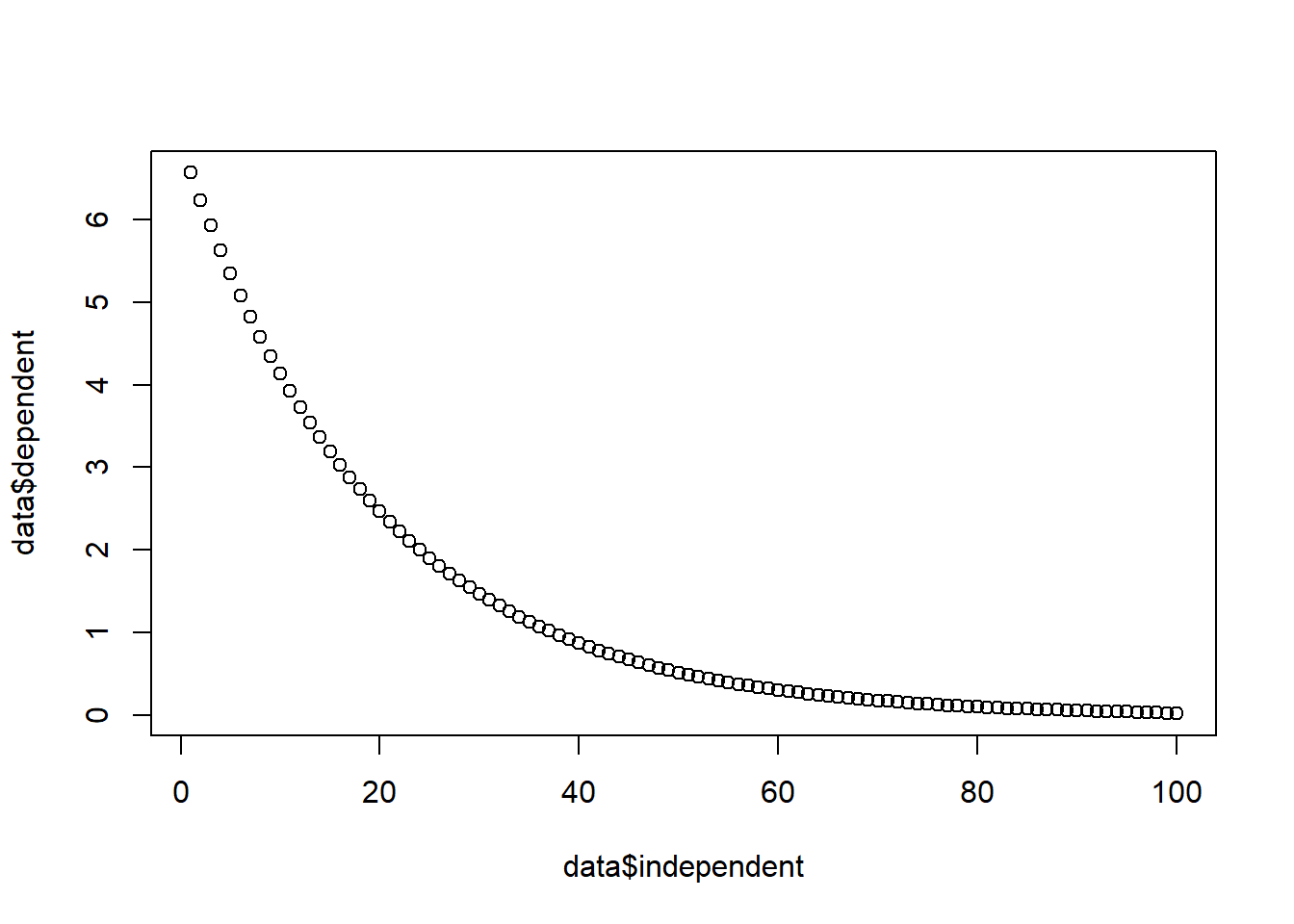
Logarithmic regression is a statistical technique used to model the relationship between a dependent variable and an independent variable when the relationship is logarithmic. In other words, it is used to model situations where the dependent variable changes at a decreasing rate as the independent variable increases.

In this blog post, we will guide you through the process of performing logarithmic regression in R, from data preparation to visualizing the results. We will also discuss how to calculate prediction intervals and plot them along with the regression line.

Step 1: Data Preparation

Before diving into the analysis, it is essential to ensure that your data is properly formatted and ready for analysis. This may involve data cleaning, checking for missing values, and handling outliers.

Step 2: Visualizing the Data

A quick scatterplot of the dependent variable versus the independent variable can provide valuable insights into the relationship between the two variables. This will help you determine if a logarithmic regression model is appropriate for your data.

# Load the data
x <- seq(from = 1, to = 100, by = 1)
y <- log(seq(from = 1000, to = 1, by = -10))
y <- y * exp(-0.05 * x)
data <- data.frame(dependent = y, independent = x)

# Create a scatterplot
plot(data$independent, data$dependent)

Step 3: Fitting the Logarithmic Regression Model

The lm() function in R can be used to fit a logarithmic regression model. The syntax for fitting a logarithmic regression model is as follows:

model <- lm(dependent ~ log(independent), data = data)

Step 4: Evaluating the Model

Once the model has been fitted, it is important to evaluate its performance. There are several metrics that can be used to evaluate the performance of a logarithmic regression model, such as the coefficient of determination (R-squared) and the mean squared error (MSE).

summary(model)


Call:
lm(formula = dependent ~ log(independent), data = data)

Residuals:
     Min       1Q   Median       3Q      Max 
-1.12938 -0.24849 -0.03559  0.23825  0.55343 

Coefficients:
                 Estimate Std. Error t value Pr(>|t|)    
(Intercept)       7.70024    0.12087   63.71   <2e-16 ***
log(independent) -1.76239    0.03221  -54.72   <2e-16 ***
---
Signif. codes:  0 '***' 0.001 '**' 0.01 '*' 0.05 '.' 0.1 ' ' 1

Residual standard error: 0.2974 on 98 degrees of freedom
Multiple R-squared:  0.9683,    Adjusted R-squared:  0.968 
F-statistic:  2994 on 1 and 98 DF,  p-value: < 2.2e-16

Step 5: Calculating Prediction Intervals

Prediction intervals provide a range of values within which we expect the true value of the dependent variable to fall for a given value of the independent variable. There are several methods for calculating prediction intervals, but one common method is to use the predict() function in R.

newdata <- data.frame(independent = seq(from = 1, to = 100, length.out = 1000))

predictions <- predict(model, 
                       newdata = newdata, 
                       interval = "prediction",
                       level = 0.95)

Step 6: Plotting the Predictions and Intervals

Plotting the predictions and intervals along with the regression line can help visualize the relationship between the variables and the uncertainty in the predictions.

plot(data$independent, data$dependent)
lines(predictions[, 1] ~ newdata$independent, lwd = 2)
matlines(newdata$independent, predictions[, 2:3], lty = 2, lwd = 2)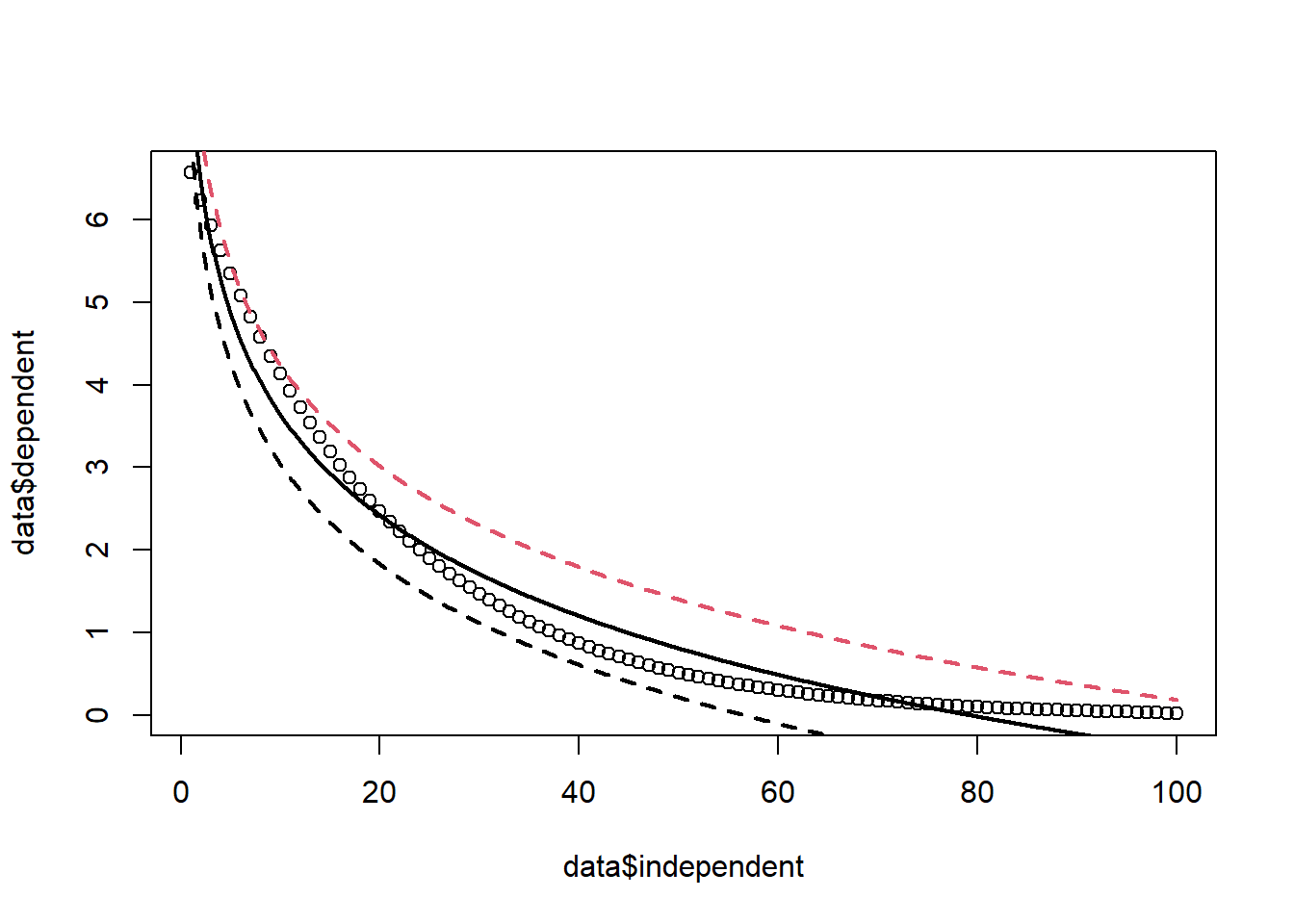

Conclusion

Logarithmic regression is a powerful statistical technique that can be used to model a variety of relationships between variables. By following the steps outlined in this blog post, you can implement logarithmic regression in R to gain valuable insights from your data.

You Try!!

We encourage you to try out logarithmic regression on your own data. Start by exploring the relationship between your variables using a scatterplot. Then, fit a logarithmic regression model using the lm() function and evaluate its performance using the summary() function. Finally, calculate prediction intervals and plot them along with the regression line to visualize the relationship between the variables and the uncertainty in the predictions.