Introduction

In the realm of statistics, power regression stands out as a versatile tool for exploring the relationship between two variables, where one variable is the power of the other. This type of regression is particularly useful when there’s an inherent nonlinear relationship between the variables, often characterized by an exponential or inverse relationship.

Power regression takes the form of y = ax^b, where:

y: The response variable, the quantity we’re trying to predict
x: The predictor variable, the quantity we’re using to make predictions
a: The intercept, the value of y when x = 1
b: The power coefficient, which determines the rate at which y changes as x increases or decreases

Steps

Step 1: Gathering the Data

To embark on our power regression journey, we’ll need some data to work with. Let’s simulate a dataset that exhibits an exponential relationship between two variables:

# Simulate data
x <- seq(1, 100, 1)
y <- 2 * x^3 + rnorm(100)

Step 2: Visualizing the Data

Before diving into the regression analysis, it’s crucial to visualize the data to gain a deeper understanding of the underlying relationship between the variables. A scatterplot can effectively reveal any patterns or trends in the data.

# Create scatterplot
plot(x, y)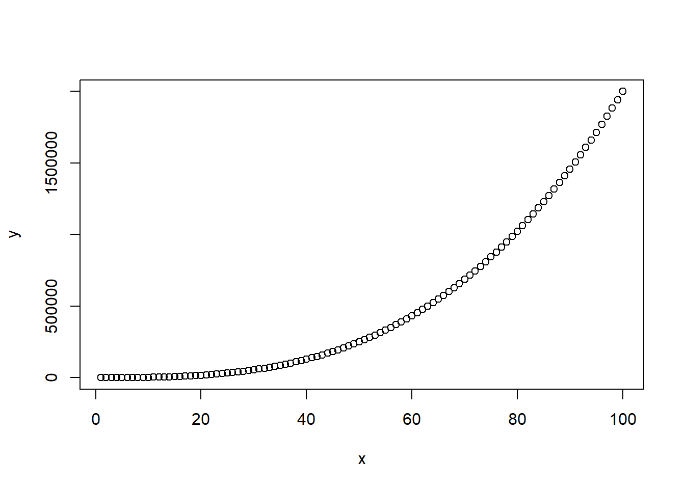

Step 3: Transforming the Data

Since power regression assumes a nonlinear relationship between the variables, we need to transform the data to fit the model’s structure. This involves taking the logarithm of both sides of the power regression equation:

# Transform data
log_y <- log(y)
log_x <- log(x)

Step 4: Fitting the Power Regression Model

Now that the data is suitably transformed, we can proceed with fitting the power regression model using the lm() function in R:

# Fit power regression model
model <- lm(log_y ~ log_x)

Step 5: Examining the Model Results

The summary() function provides valuable insights into the model’s performance, including the estimated regression coefficients, their standard errors, and the p-values associated with each coefficient.

# Summarize model results
summary(model)


Call:
lm(formula = log_y ~ log_x)

Residuals:
     Min       1Q   Median       3Q      Max 
-0.10472 -0.01800  0.00221  0.01433  0.61505 

Coefficients:
            Estimate Std. Error t value Pr(>|t|)    
(Intercept) 0.812631   0.027647   29.39   <2e-16 ***
log_x       2.969125   0.007367  403.03   <2e-16 ***
---
Signif. codes:  0 '***' 0.001 '**' 0.01 '*' 0.05 '.' 0.1 ' ' 1

Residual standard error: 0.06803 on 98 degrees of freedom
Multiple R-squared:  0.9994,    Adjusted R-squared:  0.9994 
F-statistic: 1.624e+05 on 1 and 98 DF,  p-value: < 2.2e-16

Step 6: Visualizing the Fitted Model

Visualizing the fitted model allows us to evaluate how well the model captures the underlying relationship between the variables. We can add the fitted model to the scatterplot using the predict() function (don’t forget to exponentiate!):

# Predict fitted values
fitted_values <- predict(model, newdata = data.frame(x = x),
                        interval = "prediction",
                        level = 0.95)

# Add fitted model to scatterplot
plot(x, y)
lines(x, exp(fitted_values[, 1]), col = "red")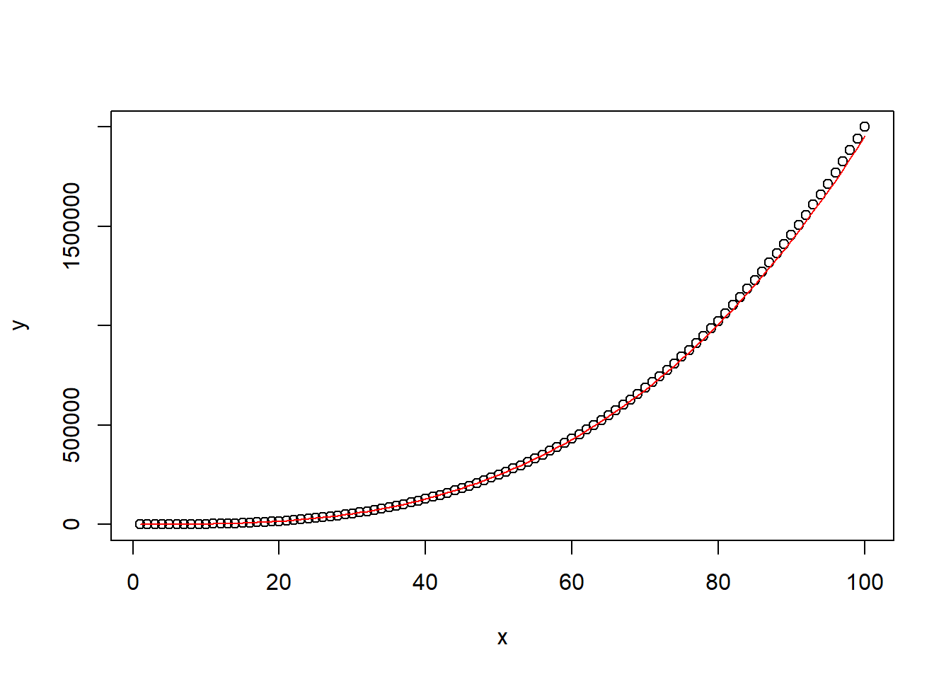

Step 7: Calculating Prediction Intervals

Prediction intervals provide a range of plausible values for the response variable at a given level of confidence. We calculated the prediction intervals using the predict() function above:

# Add fitted model to scatterplot
plot(x, y)
lines(x, exp(fitted_values[, 1]), col = "red")

# Add prediction intervals to scatterplot
lines(x, exp(fitted_values[, 2]), col = "blue", lty = 2)
lines(x, exp(fitted_values[, 3]), col = "blue", lty = 2)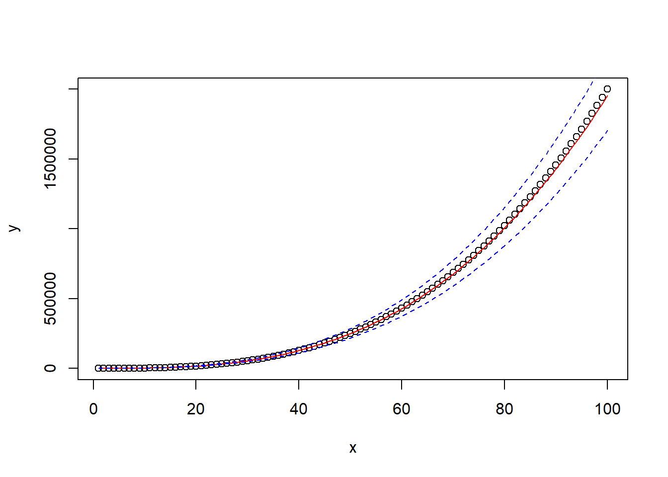

Conclusion

Power regression serves as a powerful tool for modeling nonlinear relationships between variables. By transforming the data, fitting the model, and visualizing the results, we can gain valuable insights into the underlying patterns and make informed predictions about the response variable.