Introduction

Stepwise regression is a powerful technique used to build predictive models by iteratively adding or removing variables based on statistical criteria. In R, this can be achieved using functions like step() or manually with forward and backward selection.

Example

Empty Model:

Let’s start with an empty model, an intercept only model.

intercept_model <- lm(mpg ~ 1, data = mtcars)
step(intercept_model)

Start:  AIC=115.94
mpg ~ 1


Call:
lm(formula = mpg ~ 1, data = mtcars)

Coefficients:
(Intercept)  
      20.09

In simple terms, we start with a model containing no predictors (mpg ~ 1) and iteratively add the most statistically significant variables until no improvement is observed. Since there are no predictors there is nothing to run through.

Forward Stepwise Regression:

# Initialize model
forward_model <- lm(mpg ~ ., data = mtcars)

# Forward stepwise regression
forward_model <- step(forward_model, direction = "forward", scope = formula(~ .))

Start:  AIC=70.9
mpg ~ cyl + disp + hp + drat + wt + qsec + vs + am + gear + carb

In simple terms, we start with a model containing all of the predictors (mpg ~ .) and iteratively add the most statistically significant variables until no improvement is observed.

Backward Stepwise Regression:

# Initialize a model with all predictors
backward_model <- lm(mpg ~ ., data = mtcars)

# Backward stepwise regression
backward_model <- step(backward_model, direction = "backward", trace = 0)

Here, we begin with a model including all predictors and iteratively remove the least statistically significant variables until the model no longer improves.

Both-Direction Stepwise Regression:

# Initialize a model with all predictors
both_model <- lm(mpg ~ ., data = mtcars)

# Both-direction stepwise regression
both_model <- step(both_model, direction = "both", trace = 0)

In both-direction regression, the algorithm combines both forward and backward steps, optimizing the model by adding significant variables and removing insignificant ones.

Visualizing Data and Model Fit:

Now, let’s visualize the data and model fit using base R plots.

# Scatter plot of mpg vs. hp
plot(mtcars$hp, mtcars$mpg, 
     main = "Scatter Plot of mpg vs. hp", 
     xlab = "hp", ylab = "mpg", pch = 20
     )
abline(lm(mpg ~ hp, data = mtcars), col = "black", lwd = 2)
points(sort(mtcars$hp), intercept_model$fitted.values, col = "purple", pch = 20)
points(sort(mtcars$hp), forward_model$fitted.values, col = "red", pch = 20)
points(sort(mtcars$hp), backward_model$fitted.values, col = "blue", pch = 20)
points(sort(mtcars$hp), both_model$fitted.values, col = "green", pch = 20)

legend(
  "topright", 
  legend = c(
    "Intercept Only", 
    "Forward", 
    "Backward", 
    "Both-Direction"
    ),
  col = c("red", "blue", "green"), pch = 20
)

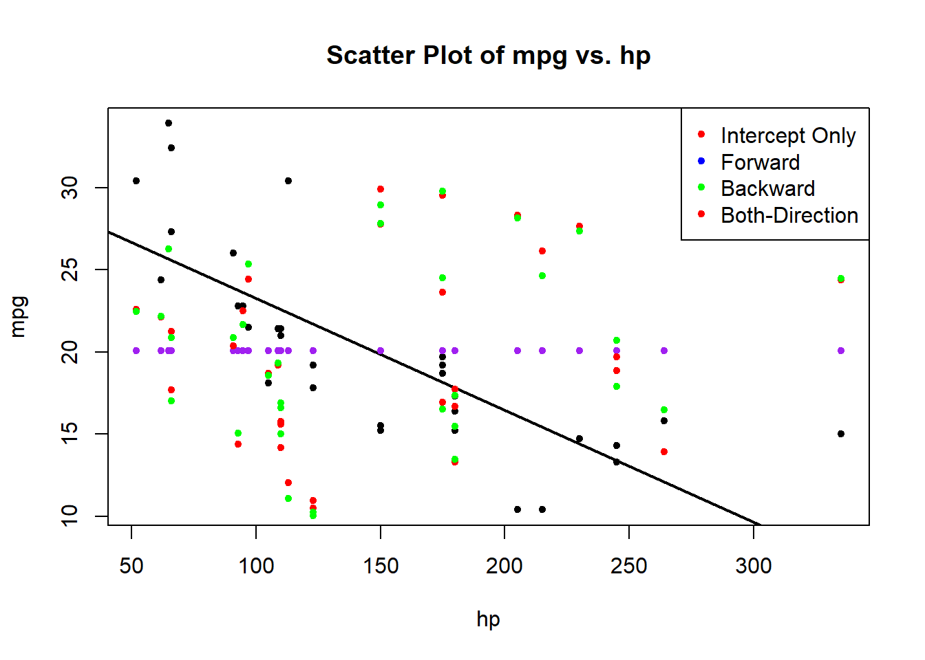
This plot displays the scatter plot of mpg against hp with fitted lines for each stepwise regression. The colors correspond to the models created earlier.

Visualizing Residuals:

# Residual plots for each model
par(mfrow = c(2, 2))

# Intercept Model
plot(intercept_model$residuals, main = "Intercept Residuals", ylab = "Residuals")

# Forward stepwise regression residuals
plot(forward_model$residuals, main = "Forward Residuals", ylab = "Residuals")

# Backward stepwise regression residuals
plot(backward_model$residuals, main = "Backward Residuals", ylab = "Residuals")

# Both-direction stepwise regression residuals
plot(both_model$residuals, main = "Both-Direction Residuals", ylab = "Residuals")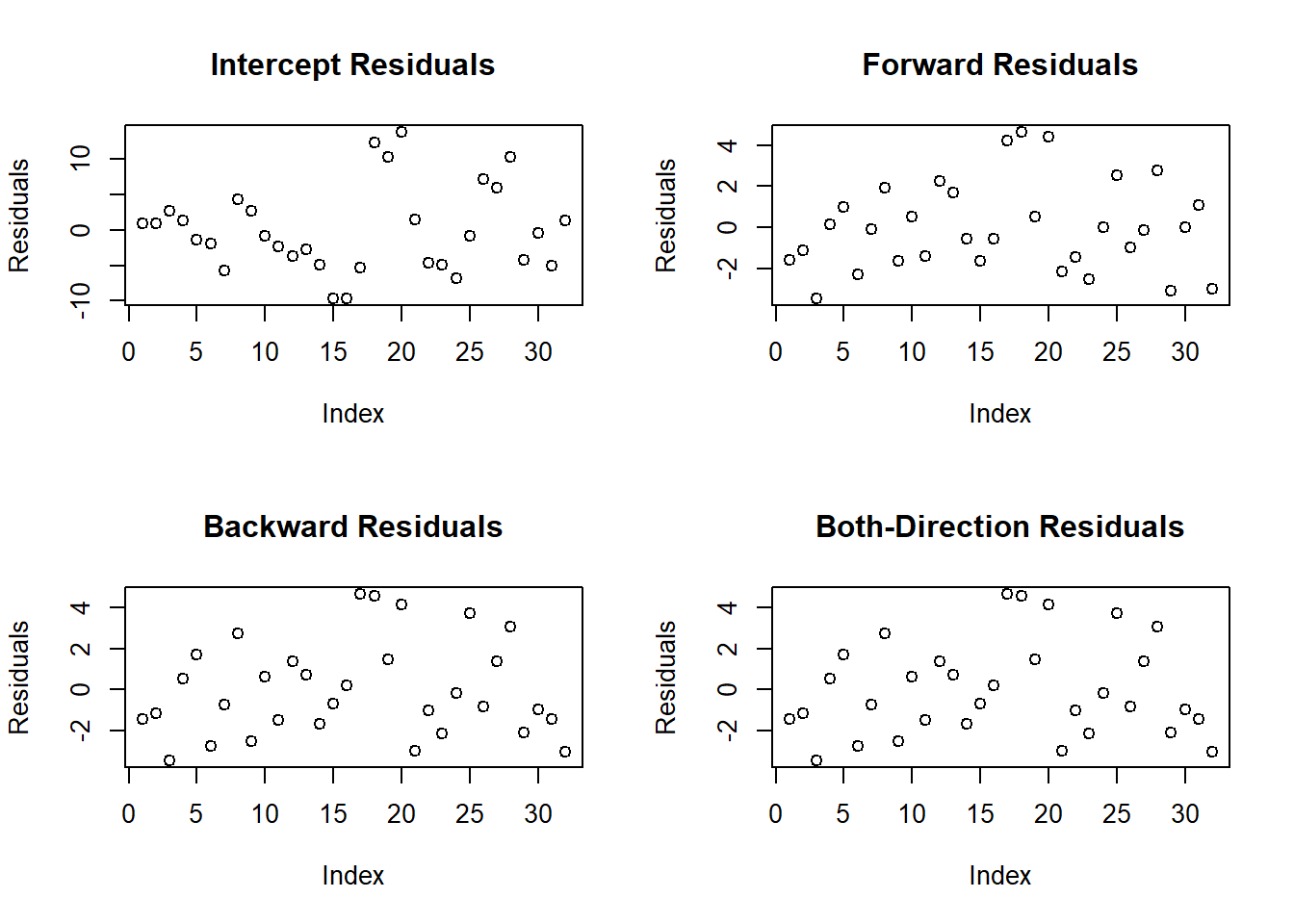

par(mfrow = c(1, 1))

These plots help assess how well the models fit the data by examining the residuals.

Conclusion

Stepwise regression is a valuable tool, but it’s crucial to interpret results cautiously and be aware of potential pitfalls.