Introduction

If you’re a data enthusiast diving into the world of regression analysis in R, you’ve likely encountered the challenges of managing code complexity and juggling different modeling engines. The good news is that there’s a powerful tool to streamline your regression workflow – the tidyAML R package.

Getting Started with TidyAML

Before we dive into the script, let’s make sure you have the necessary libraries installed. Fire up your R console and install the tidyAML package along with its dependencies:

install.packages("tidyAML")

Now, let’s explore a script that leverages tidyAML for quick and efficient regression analysis. Here’s a breakdown of the key components:

Intial Setup

library(tidyAML)
library(tidyverse)
library(tidymodels)
library(multilevelmod)
library(earth)
library(randomForest)
library(rpart)
library(lightgbm)
library(baguette)
library(bonsai)
library(gee)

tidymodels_prefer()

Setting Up the Recipe

df <- mtcars
recipe <- recipe(mpg ~ ., data = df)

In this snippet, we’re creating a recipe for our regression analysis. The response variable (mpg) is modeled against all other variables in the mtcars dataset.

Fast Regression with TidyAML

fr_tbl <- fast_regression(
  .data = df,
  .rec_obj = recipe,
  .parsnip_fns = c("linear_reg", "mars", "bag_mars", "rand_forest",
                   "boost_tree", "bag_tree"),
  .parsnip_eng = c("lm", "gee", "glm", "gls", "earth", "rpart", "lightgbm")
)

This is where the magic happens. The fast_regression function performs regression using various modeling functions (linear_reg, mars, etc.) and engines (lm, gee, etc.) specified. It’s a versatile approach to quickly explore different models.

Visualizing Residuals

fr_tbl |>
  mutate(res = map(fitted_wflw, \(x) x |> 
                     broom::augment(new_data = df))) |>
  unnest(cols = res) |>
  mutate(pfe = paste0(.parsnip_engine, " - ", .parsnip_fns)) |>
  mutate(.res = mpg - .pred) |>
  ggplot(aes(x = pfe, y = .res, fill = pfe)) +
    geom_boxplot() +
    theme_minimal() +
    labs(title = "Residuals by Fitted Model",
       subtitle = "Residuals are mpg - .pred",
       x = "Model",
       y = "Residuals",
       fill = "Engine + Function") +
  theme(axis.text.x = element_text(angle = 45, hjust = 1))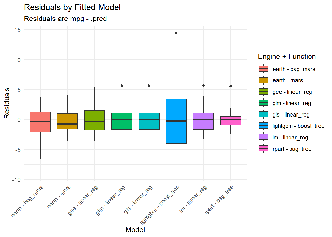

This block of code generates a boxplot visualizing residuals by model. Residuals are the differences between observed and predicted values. The plot helps you assess how well your models are performing.

Try It Yourself!

Now that you’ve seen the power of tidyAML in action, it’s time to try it yourself. Install the package, load your data, and adapt the script to your specific use case. TidyAML provides a clean and efficient way to explore different regression models, making your analysis more manageable and insightful.

install.packages("tidyAML")
library(tidyAML)
# Your data loading and analysis code here

Happy coding, and may your regression analyses be tidy and insightful!