Introduction

Ever felt those data points were a bit too jittery? Smoothing out trends and revealing underlying patterns is a breeze with rolling averages in R. Ready to roll? Let’s dive in!

Rolling with the ‘zoo’

Meet the ‘zoo’ package, your trusty companion for time series data wrangling. It’s got a handy function called ‘rollmean’ that handles those rolling averages with ease.

Installing and Loading

# install.packages("zoo")  # Grab it if you haven't already
library(zoo)  # Bring it into your workspace

Example

Creating a Simple Time Series

set.seed(123)  # Set seed for reproducibility (optional
# Let's imagine some daily sales data
sales <- trunc(runif(112, min = 100, max = 500))  # Generate some random sales
days <- as.Date(1:112, origin = "2022-12-31")  # Add some dates!
data_zoo <- zoo(sales, days)  # Convert to a zoo object

Calculating Rolling Averages

# Say we want a 7-day rolling average:
rolling_avg7 <- rollmean(data_zoo, k = 7)
rolling_avg7_left <- rollmean(data_zoo, k = 7, align = "left")
rolling_avg7_right <- rollmean(data_zoo, k = 7, align = "right")

# How about a 28-day one?
rolling_avg28 <- rollmean(data_zoo, k = 28)
rolling_avg28_left <- rollmean(data_zoo, k = 28, align = "left")
rolling_avg28_right <- rollmean(data_zoo, k = 28, align = "right")

Visualizing the Smoothness

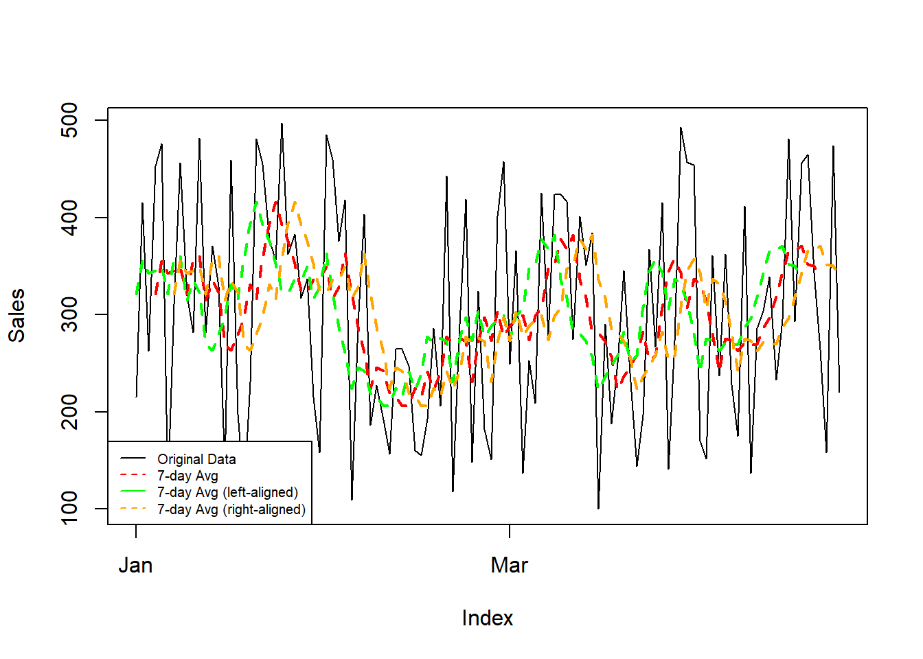
plot(data_zoo, type = "l", col = "black", lwd = 1, ylab = "Sales")
lines(rolling_avg7, col = "red", lwd = 2, lty = 2)
lines(rolling_avg7_left, col = "green", lwd = 2, lty = 2)
lines(rolling_avg7_right, col = "orange", lwd = 2, lty = 2)
legend(
  "bottomleft", 
  legend = c(
    "Original Data", "7-day Avg", "7-day Avg (left-aligned)", 
    "7-day Avg (right-aligned)"
    ),
  col = c("black", "red", "green", "orange"), 
  lwd = 1, lty = 1:2,
  cex = 0.628
  )

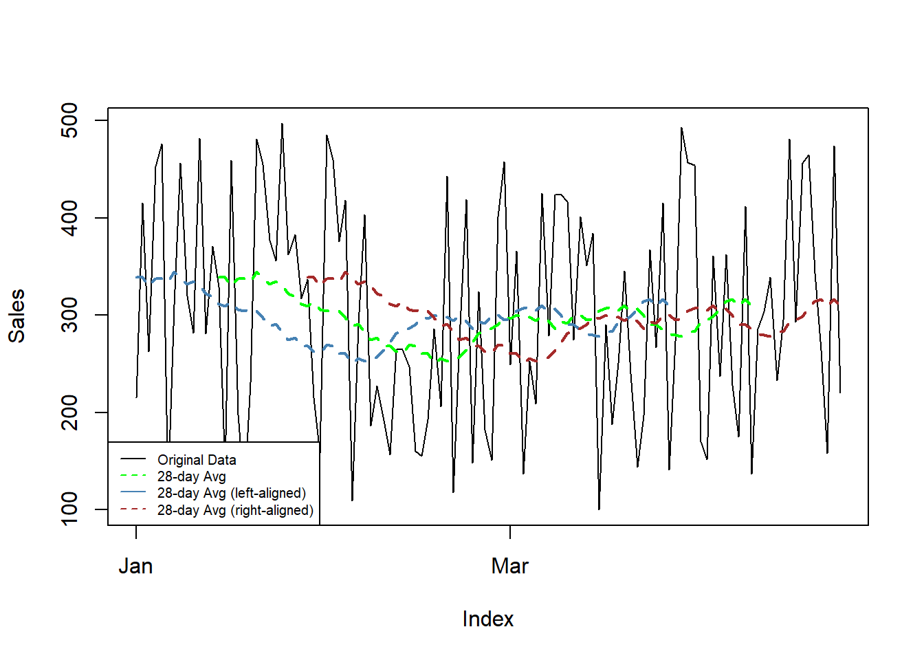
plot(data_zoo, type = "l", col = "black", lwd = 1, ylab = "Sales")
lines(rolling_avg28, col = "green", lwd = 2, lty = 2)
lines(rolling_avg28_left, col = "steelblue", lwd = 2, lty = 2)
lines(rolling_avg28_right, col = "brown", lwd = 2, lty = 2)
legend(
  "bottomleft", 
  legend = c(
    "Original Data", "28-day Avg", "28-day Avg (left-aligned)", 
    "28-day Avg (right-aligned)"
    ),
  col = c("black", "green", "steelblue", "brown"), 
  lwd = 1, lty = 1:2,
  cex = 0.628
  )

Experimenting and Interpreting

Play with different ‘k’ values to see how they affect the smoothness. Remember, larger ‘k’ means more smoothing, but potential loss of detail.

Your Turn to Roll!

Grab your data and start exploring rolling averages! It’s a powerful tool to uncover hidden patterns and trends. Share your discoveries and join the rolling conversation!