Estimating Chi-Square Distribution Parameters Using R

code
rtip
operations
glue
unglue
Author

Steven P. Sanderson II, MPH

Published

April 15, 2024

Introduction

In the world of statistics and data analysis, understanding and accurately estimating the parameters of probability distributions is crucial. One such distribution is the chi-square distribution, often encountered in various statistical analyses. In this blog post, we’ll dive into how we can estimate the degrees of freedom (“df”) and the non-centrality parameter (“ncp”) of a chi-square distribution using R programming language.

The Chi-Square Distribution

The chi-square distribution is a continuous probability distribution that arises in the context of hypothesis testing and confidence interval estimation. It is commonly used in goodness-of-fit tests, tests of independence, and tests of homogeneity.

The distribution has two main parameters: - Degrees of Freedom (df): This parameter determines the shape of the chi-square distribution. It represents the number of independent variables in a statistical test. - Non-Centrality Parameter (ncp): This parameter determines the deviation of the distribution from a null hypothesis. It’s particularly relevant in non-central chi-square distributions.

The Goal: Estimating Parameters

Our goal is to create a function within the TidyDensity package that can estimate the df and ncp parameters of a chi-square distribution based on a vector of observed data. Let’s walk through the steps involved in achieving this.

Working Example

Setting the Stage: Libraries and Data

First, we load the necessary libraries: tidyverse for data manipulation and bbmle for maximum likelihood estimation. We then generate a grid of parameters (degrees of freedom and non-centrality parameter) and sample sizes to create a diverse set of chi-square distributed data.

# Load libraries
library(tidyverse)
library(bbmle)

# Data ----
# Make parameters and grid
df <- 1:10
ncp <- 1:10
n <- runif(10, 250, 500) |> trunc()
param_grid <- expand_grid(n = n, df = df, ncp = ncp)

head(param_grid)
# A tibble: 6 × 3
      n    df   ncp
  <dbl> <int> <int>
1   284     1     1
2   284     1     2
3   284     1     3
4   284     1     4
5   284     1     5
6   284     1     6

Function Exploration: Unveiling the Estimation Process

The core of our exploration lies in several functions designed to estimate the chi-square parameters:

dof/k Functions: These functions focus on estimating the degrees of freedom (df) using different approaches:

  • mean_x: Calculates the mean of the data.
  • mean_minus_1: Subtracts 1 from the mean.
  • var_div_2: Divides the variance of the data by 2.
  • length_minus_1: Subtracts 1 from the length of the data.

ncp Functions: These functions aim to estimate the non-centrality parameter (ncp) using various methods:

  • mean_minus_mean_minus_1: A seemingly trivial calculation that serves as a baseline.
  • ie_mean_minus_var_div_2: Subtracts half the variance from the mean, ensuring the result is non-negative.
  • ie_optim: Utilizes optimization techniques to find the ncp that maximizes the likelihood of observing the data.
  • estimate_chisq_params: This is the main function that employs maximum likelihood estimation (MLE) via the bbmle package to estimate both df and ncp simultaneously. It defines a negative log-likelihood function based on the chi-square distribution and uses mle2 to find the parameter values that minimize this function.
# Functions ----
# functions to estimate the parameters of a chisq distribution
# dof
mean_x <- function(x) mean(x)
mean_minus_1 <- function(x) mean(x) - 1
var_div_2 <- function(x) var(x) / 2
length_minus_1 <- function(x) length(x) - 1
# ncp
mean_minus_mean_minus_1 <- function(x) mean(x) - (mean(x) - 1)
ie_mean_minus_var_div_2 <- function(x) ifelse((mean(x) - (var(x) / 2)) < 0, 0, mean(x) - var(x)/2)
ie_optim <- function(x) optim(par = 0,
                             fn = function(ncp) {
                               -sum(dchisq(x, df = var(x)/2, ncp = ncp, log = TRUE))
                             },
                             method = "Brent",
                             lower = 0,
                             upper = 10 * var(x)/2)$par
# both
estimate_chisq_params <- function(data) {
  # Negative log-likelihood function
  negLogLik <- function(df, ncp) {
    -sum(dchisq(data, df = df, ncp = ncp, log = TRUE))
  }
  
  # Initial values (adjust based on your data if necessary)
  start_vals <- list(df = trunc(var(data)/2), ncp = trunc(mean(data)))
  
  # MLE using bbmle
  mle_fit <- bbmle::mle2(negLogLik, start = start_vals)
  # Return estimated parameters as a named vector
  df <- dplyr::tibble(
    est_df = coef(mle_fit)[1],
    est_ncp = coef(mle_fit)[2]
  )
  return(df)
}

safe_estimates <- {
  purrr::possibly(
    estimate_chisq_params,
    otherwise = NA_real_,
    quiet = TRUE
  )
}

Simulating and Evaluating: Putting the Functions to the Test

To assess the performance of our functions, we simulate chi-square data using the parameter grid and apply each function to estimate the parameters. We then compare these estimates to the true values and visualize the results using boxplots.

# Simulate data ----
set.seed(123)
dff <- param_grid |>
  mutate(x = pmap(pick(everything()), match.fun("rchisq"))) |>
  mutate(
    safe_est_parms = map(x, safe_estimates),
    dfa = map_dbl(x, mean_minus_1),
    dfb = map_dbl(x, var_div_2),
    dfc = map_dbl(x, length_minus_1),
    ncpa = map_dbl(x, mean_minus_mean_minus_1),
    ncpb = map_dbl(x, ie_mean_minus_var_div_2),
    ncpc = map_dbl(x, ie_optim)
  ) |>
  select(-x) |>
  filter(map_lgl(safe_est_parms, ~ any(is.na(.x))) == FALSE) |>
  unnest(cols = safe_est_parms) |>
  mutate(
    dfa_resid = dfa - df,
    dfb_resid = dfb - df,
    dfc_resid = dfc - df,
    dfd_resid = est_df - df,
    ncpa_resid = ncpa - ncp,
    ncpb_resid = ncpb - ncp,
    ncpc_resid = ncpc - ncp,
    ncpd_resid = est_ncp - ncp
  )

glimpse(dff)
Rows: 987
Columns: 19
$ n          <dbl> 284, 284, 284, 284, 284, 284, 284, 284, 284, 284, 284, 284,…
$ df         <int> 1, 1, 1, 1, 1, 1, 1, 1, 1, 1, 2, 2, 2, 2, 2, 2, 2, 2, 2, 2,…
$ ncp        <int> 1, 2, 3, 4, 5, 6, 7, 8, 9, 10, 1, 2, 3, 4, 5, 6, 7, 8, 9, 1…
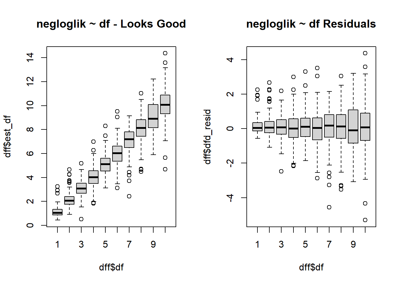
$ est_df     <dbl> 1.1770904, 0.9905994, 0.9792179, 0.7781877, 1.5161669, 0.82…
$ est_ncp    <dbl> 0.7231638, 1.9462325, 3.0371756, 4.2347494, 3.7611119, 6.26…
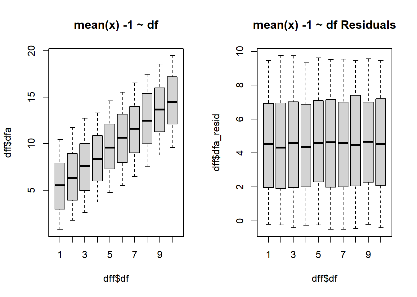
$ dfa        <dbl> 0.9050589, 1.9826153, 3.0579375, 4.0515312, 4.2022289, 6.15…
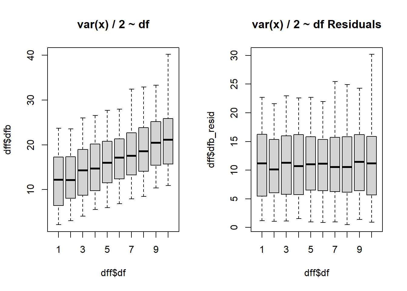
$ dfb        <dbl> 2.626501, 5.428382, 7.297746, 9.265272, 8.465838, 14.597976…
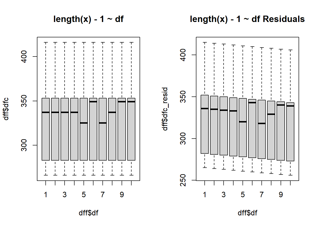
$ dfc        <dbl> 283, 283, 283, 283, 283, 283, 283, 283, 283, 283, 283, 283,…
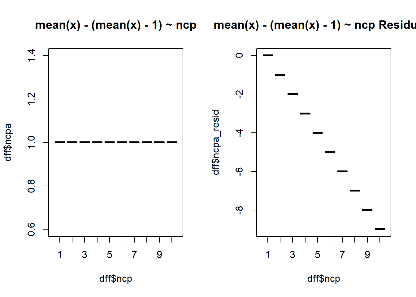
$ ncpa       <dbl> 1, 1, 1, 1, 1, 1, 1, 1, 1, 1, 1, 1, 1, 1, 1, 1, 1, 1, 1, 1,…
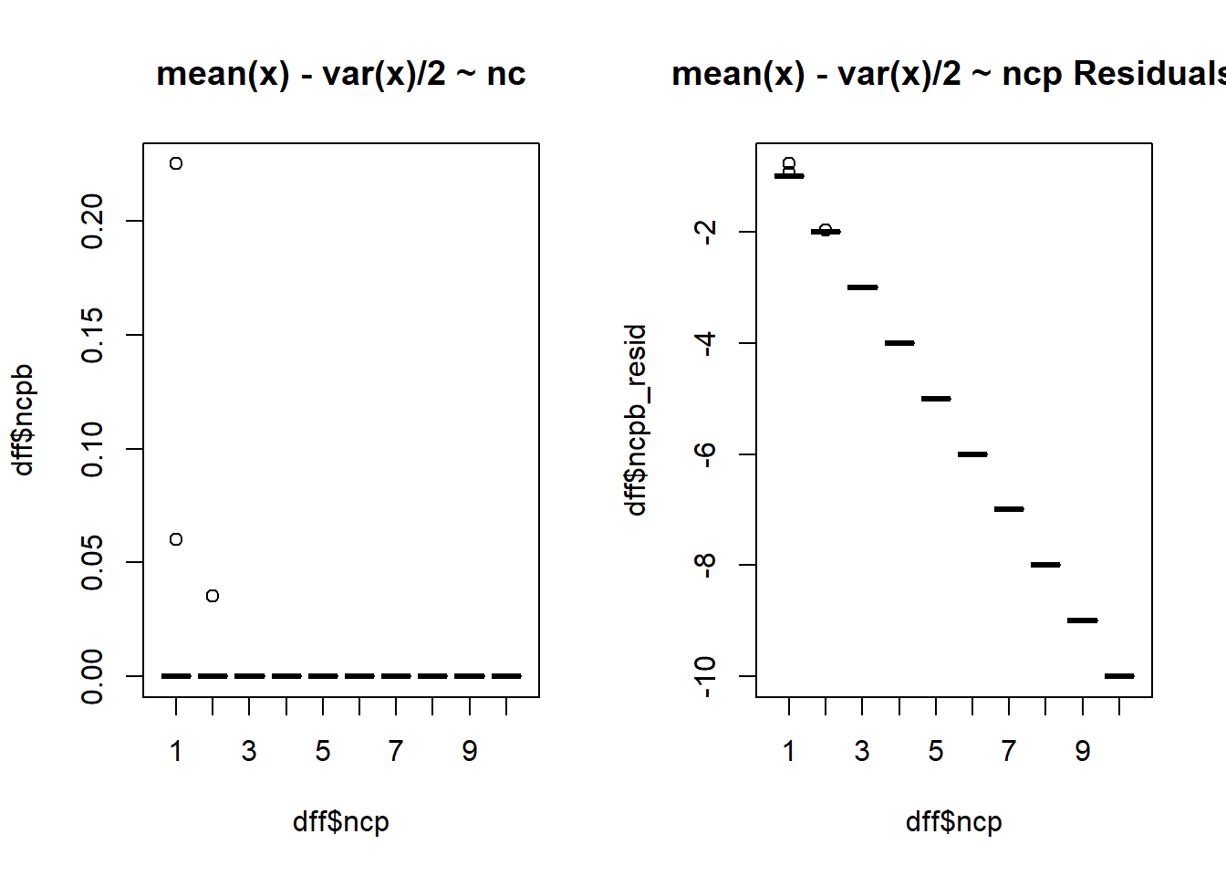
$ ncpb       <dbl> 0, 0, 0, 0, 0, 0, 0, 0, 0, 0, 0, 0, 0, 0, 0, 0, 0, 0, 0, 0,…
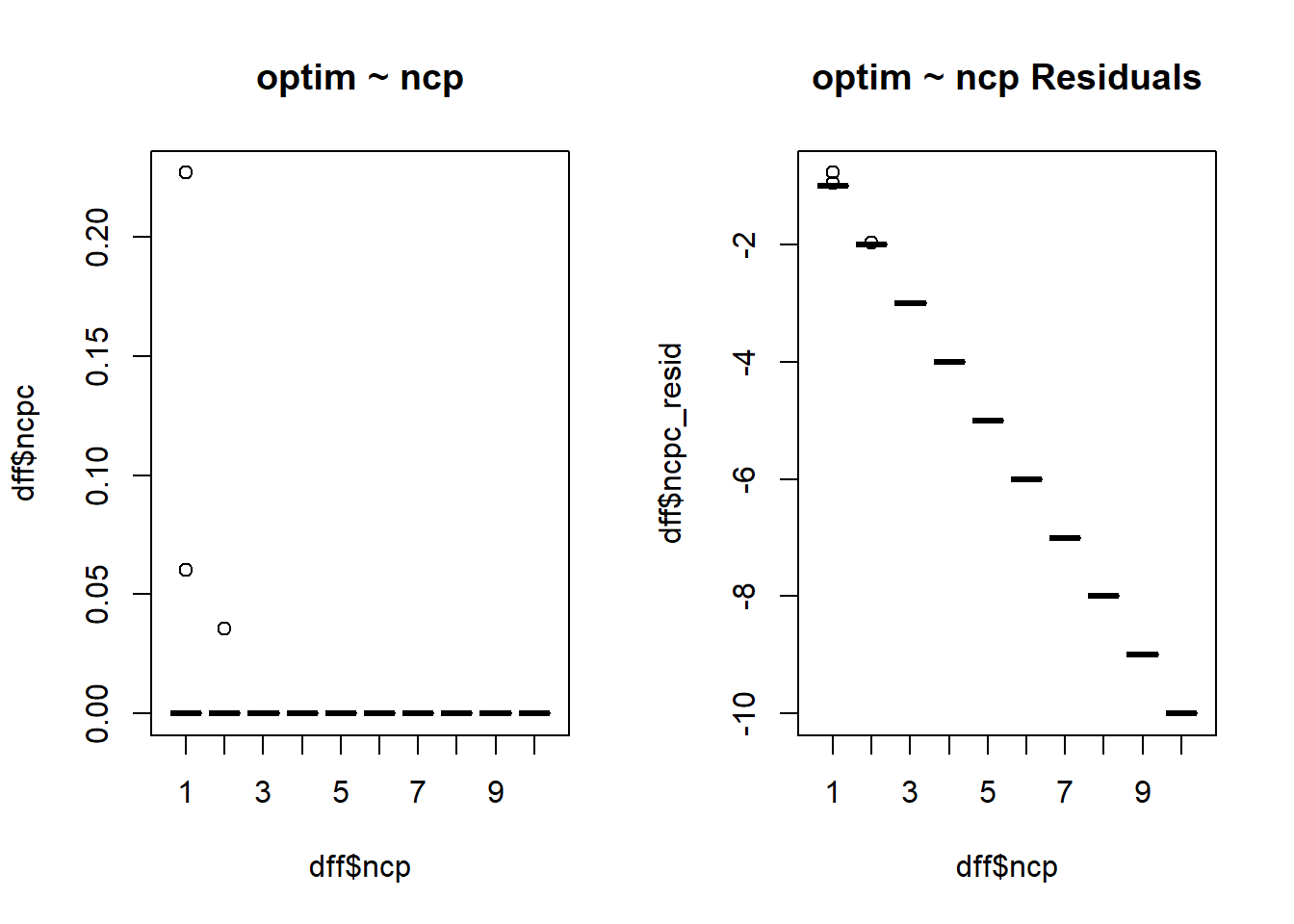
$ ncpc       <dbl> 5.382789e-09, 8.170550e-09, 6.017177e-09, 8.618892e-09, 7.7…
$ dfa_resid  <dbl> -0.09494109, 0.98261533, 2.05793748, 3.05153121, 3.20222890…
$ dfb_resid  <dbl> 1.626501, 4.428382, 6.297746, 8.265272, 7.465838, 13.597976…
$ dfc_resid  <dbl> 282, 282, 282, 282, 282, 282, 282, 282, 282, 282, 281, 281,…
$ dfd_resid  <dbl> 0.177090434, -0.009400632, -0.020782073, -0.221812344, 0.51…
$ ncpa_resid <dbl> 0, -1, -2, -3, -4, -5, -6, -7, -8, -9, 0, -1, -2, -3, -4, -…
$ ncpb_resid <dbl> -1, -2, -3, -4, -5, -6, -7, -8, -9, -10, -1, -2, -3, -4, -5…
$ ncpc_resid <dbl> -1, -2, -3, -4, -5, -6, -7, -8, -9, -10, -1, -2, -3, -4, -5…
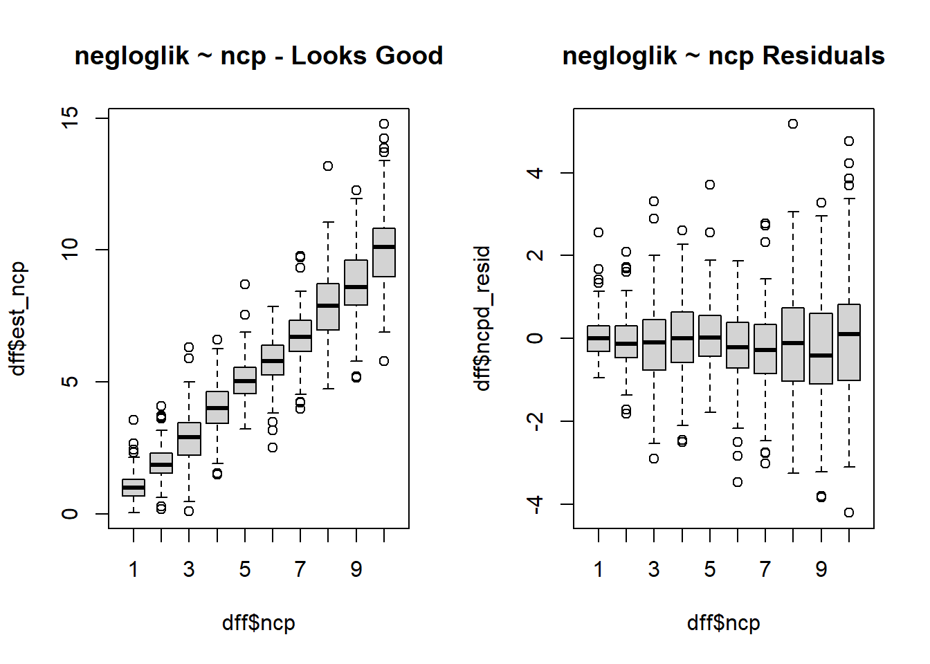
$ ncpd_resid <dbl> -0.27683618, -0.05376753, 0.03717560, 0.23474943, -1.238888…

Visual Insights: Assessing Estimation Accuracy

The boxplots reveal interesting insights:

par(mfrow = c(1, 2))
boxplot(dff$dfa ~ dff$df, main = "mean(x) -1 ~ df")
boxplot(dff$dfa_resid ~ dff$df, main = "mean(x) -1 ~ df Residuals")

par(mfrow = c(1, 1))

par(mfrow = c(1, 2))
boxplot(dff$dfb ~ dff$df, main = "var(x) / 2 ~ df")
boxplot(dff$dfb_resid ~ dff$df, main = "var(x) / 2 ~ df Residuals")

par(mfrow = c(1, 1))

par(mfrow = c(1, 2))
boxplot(dff$dfc ~ dff$df, main = "length(x) - 1 ~ df")
boxplot(dff$dfc_resid ~ dff$df, main = "length(x) - 1 ~ df Residuals")

par(mfrow = c(1, 1))

par(mfrow = c(1, 2))
boxplot(dff$est_df ~ dff$df, main = "negloglik ~ df - Looks Good")
boxplot(dff$dfd_resid ~ dff$df, main = "negloglik ~ df Residuals")

par(mfrow = c(1, 1))

par(mfrow = c(1, 2))
boxplot(dff$ncpa ~ dff$ncp, main = "mean(x) - (mean(x) - 1) ~ ncp")
boxplot(dff$ncpa_resid ~ dff$ncp, main = "mean(x) - (mean(x) - 1) ~ ncp Residuals")

par(mfrow = c(1, 1))

par(mfrow = c(1, 2))
boxplot(dff$ncpb ~ dff$ncp, main = "mean(x) - var(x)/2 ~ nc")
boxplot(dff$ncpb_resid ~ dff$ncp, main = "mean(x) - var(x)/2 ~ ncp Residuals")

par(mfrow = c(1, 1))

par(mfrow = c(1, 2))
boxplot(dff$ncpc ~ dff$ncp, main = "optim ~ ncp")
boxplot(dff$ncpc_resid ~ dff$ncp, main = "optim ~ ncp Residuals")

par(mfrow = c(1, 1))

par(mfrow = c(1, 2))
boxplot(dff$est_ncp ~ dff$ncp, main = "negloglik ~ ncp - Looks Good")
boxplot(dff$ncpd_resid ~ dff$ncp, main = "negloglik ~ ncp Residuals")

par(mfrow = c(1, 1))

df Estimation:

  • mean_x - 1 and var(x) / 2 show potential as df estimators but exhibit bias depending on the true df value.
  • length(x) - 1 performs poorly, consistently underestimating df.
  • The MLE approach from estimate_chisq_params demonstrates the most accurate and unbiased estimates across different df values.

ncp Estimation:

  • The simple methods (mean(x) - mean(x) - 1 and mean(x) - var(x) / 2) show substantial bias and variability.
  • The optimization-based method (optim) performs better but still exhibits some bias.
  • The MLE approach again emerges as the most reliable option, providing accurate and unbiased estimates across various ncp values.

Conclusion: The Power of Maximum Likelihood

Our exploration highlights the effectiveness of MLE in estimating the parameters of a chi-square distribution. The estimate_chisq_params function, utilizing the bbmle package, provides a robust and accurate solution for this task. This function will be a valuable addition to the TidyDensity package, empowering users to delve deeper into the analysis of chi-square distributed data.

Stay tuned for further developments and exciting additions to the TidyDensity package!