Introduction

In the area of statistical modeling and Bayesian inference, Markov Chain Monte Carlo (MCMC) methods are indispensable tools for tackling complex problems. The new tidy_mcmc_sampling() function in the TidyDensity R package simplifies MCMC sampling and visualization, making it accessible to a broader audience of data enthusiasts and analysts.

Understanding MCMC

Before we dive into the practical use of tidy_mcmc_sampling(), let’s briefly discuss why MCMC is valuable. MCMC methods are particularly useful when dealing with Bayesian statistics, where exact analytical solutions are challenging or impossible due to the complexity of the models involved.

MCMC allows us to draw samples from a probability distribution, especially in cases where direct sampling is impractical. This is achieved by constructing a Markov chain that converges to the desired distribution after a sufficient number of iterations. Once converged, these samples can provide insights into the posterior distribution of parameters, allowing us to make probabilistic inferences.

Introducing `tidy_mcmc_sampling()`

The tidy_mcmc_sampling() function in TidyDensity harnesses the power of MCMC sampling and presents the results in a tidy format, facilitating further analysis and visualization. Let’s explore its usage and capabilities.

Usage Example

Suppose we have a dataset data that we want to analyze using MCMC sampling:

library(TidyDensity)

# Generate MCMC samples
set.seed(123)
data <- rnorm(100)
result <- tidy_mcmc_sampling(data, .fns = "median", .cum_fns = "cmedian")
result

$mcmc_data
# A tibble: 4,000 × 3
   sim_number name                 value
   <fct>      <fct>                <dbl>
 1 1          .sample_median    -0.0285 
 2 1          .cum_stat_cmedian -0.0285 
 3 2          .sample_median     0.239  
 4 2          .cum_stat_cmedian  0.105  
 5 3          .sample_median     0.00576
 6 3          .cum_stat_cmedian  0.00576
 7 4          .sample_median    -0.0357 
 8 4          .cum_stat_cmedian -0.0114 
 9 5          .sample_median    -0.111  
10 5          .cum_stat_cmedian -0.0285 
# ℹ 3,990 more rows

$plt

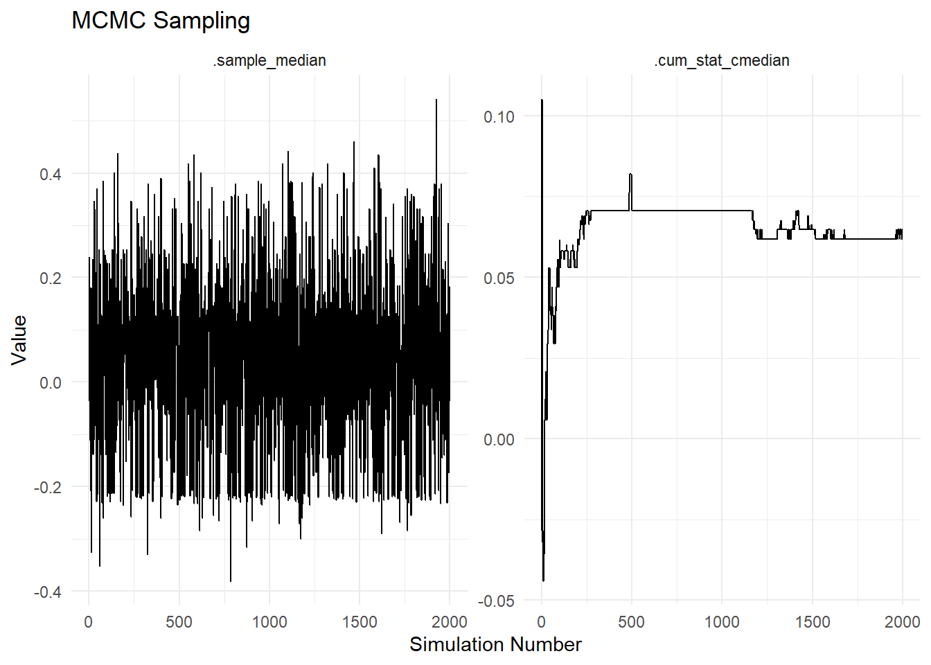
In this example: - We generate 100 random normal values using rnorm(100). - The tidy_mcmc_sampling() function is then applied to this data, specifying that we want to compute the median ("median") of each MCMC sample and the cumulative median ("cmedian") across all samples, here the default sample size is 2000.

Key Arguments

.x: The input data vector for MCMC sampling.
.fns: A character vector specifying the function(s) to apply to each MCMC sample. By default, it computes the mean ("mean"), but you can customize this to any function that makes sense for your analysis.
.cum_fns: A character vector specifying the function(s) to apply to the cumulative MCMC samples. The default is to compute the cumulative mean ("cmean"), but you can change this based on your requirements.
.num_sims: The number of MCMC simulations to run. More simulations generally lead to more accurate results but can be computationally expensive. The default is 2000.

Visualizing Results

The tidy_mcmc_sampling() function not only returns tidy data but also generates a plot to visualize the MCMC samples and cumulative statistics. This visualization is essential for understanding the distribution of samples and how they evolve over iterations.

Try It Yourself!

If you’re intrigued by the capabilities of MCMC and want to explore it in your data analysis workflow, I encourage you to try out tidy_mcmc_sampling() with your own datasets and custom functions. Experiment with different parameters and visualize the results to gain deeper insights into your data.

In conclusion, tidy_mcmc_sampling() extends the functionality of TidyDensity by offering a user-friendly interface for conducting MCMC sampling and analysis. Whether you’re new to Bayesian statistics or a seasoned practitioner, this function can streamline your workflow and enhance your understanding of complex datasets. Give it a spin and unlock new possibilities in your data exploration journey!