This tutorial explains how to use R’s diff() function to calculate differences between consecutive values in your data. You’ll learn the basic syntax, see practical examples with vectors and data frames, and understand common applications and pitfalls. All visualizations use base R graphics with code samples.

What is diff() and What Does It Do?

The diff() function in R calculates the differences between consecutive elements in a vector, data frame, or time series. It subtracts each element from the next one, giving you a result that shows how values change from one position to the next.

Basic Syntax and Parameters

diff(x, lag = 1, differences = 1, ...)

Here’s what each parameter means:

x: The input data (vector, data frame, time series)
lag: How many positions to look back when calculating differences (default is 1)
differences: How many times to apply the differencing operation (default is 1)
…: Additional arguments for specific methods

Simple Vector Examples

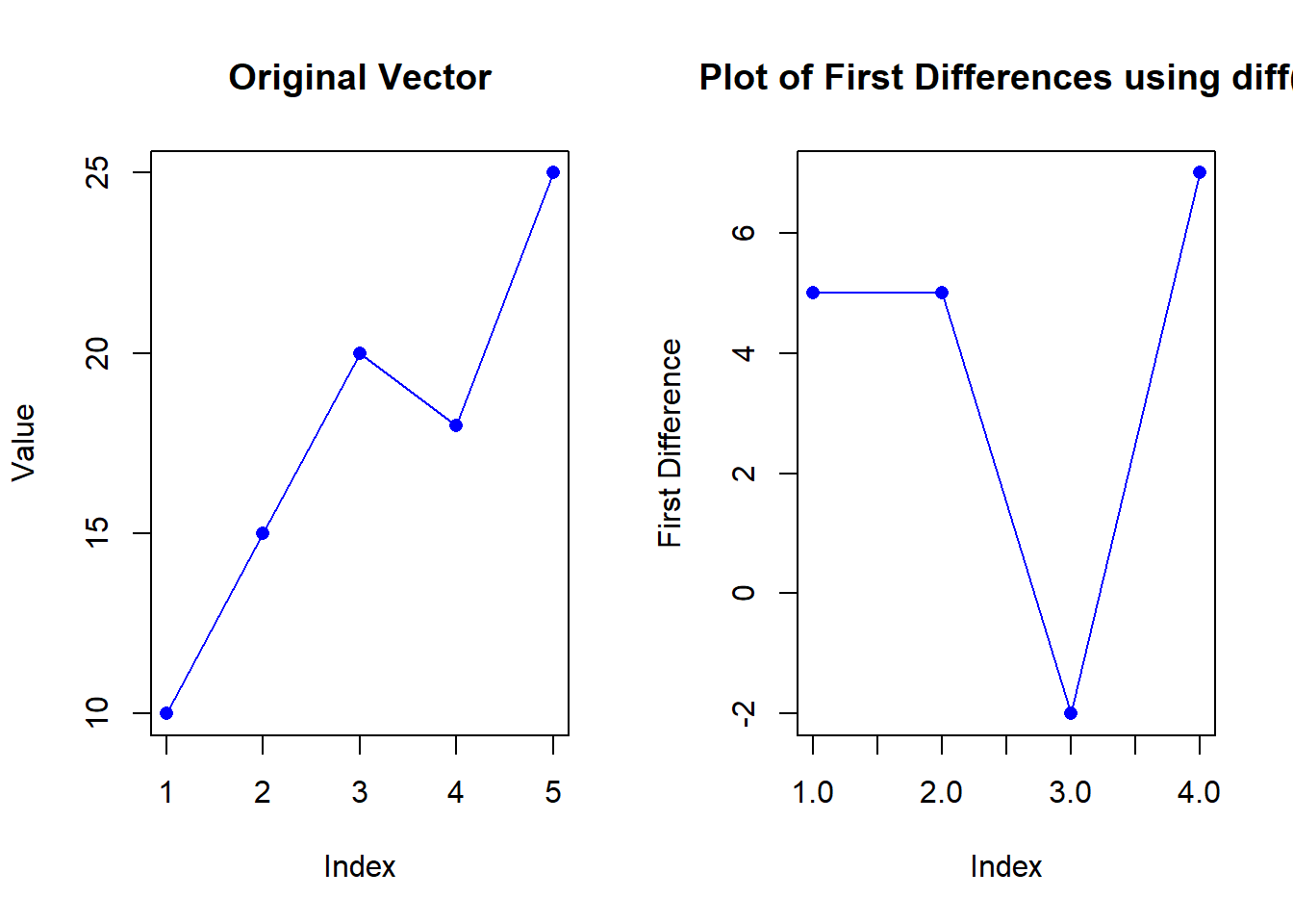
Let’s start with a basic example using a numeric vector:

# Create a vector
x <- c(10, 15, 20, 18, 25)

# Calculate differences
dx <- diff(x)
print(dx)

[1]  5  5 -2  7

# Output: 5 5 -2 7

par(mfrow = c(1, 2))
# Plot the differences using base R
plot(x, type = "o", col = "blue", pch = 16,
     xlab = "Index", ylab = "Value",
     main = "Original Vector")

plot(dx, type = "o", col = "blue", pch = 16,
     xlab = "Index", ylab = "First Difference",
     main = "Plot of First Differences using diff()")

par(mfrow = c(1, 1))

The function calculates: - 15 - 10 = 5 - 20 - 15 = 5 - 18 - 20 = -2 - 25 - 18 = 7

Working with Data Frames

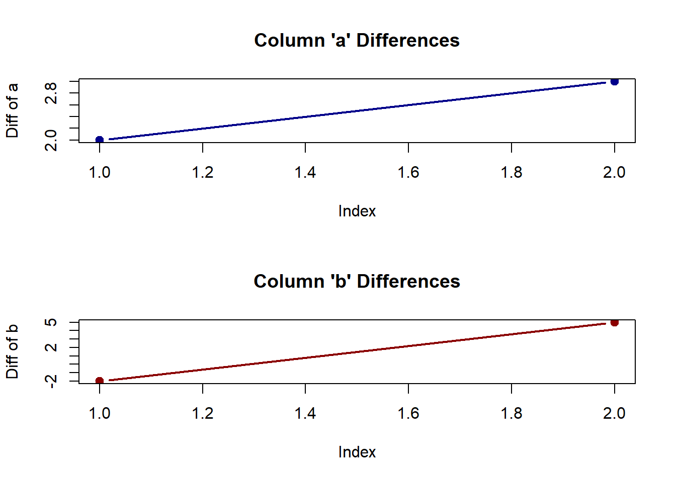
When you apply diff() to a data frame, it calculates differences for each column separately:

# Create a data frame
df <- data.frame(a = c(2, 4, 7), b = c(5, 3, 8))

# Calculate differences
diff_df <- diff(as.matrix(df)) |> as.data.frame()
print(diff_df)

  a  b
1 2 -2
2 3  5

# Plot differences for each column
par(mfrow = c(2, 1))  # Set up 2 plots stacked vertically

# Plot column 'a' differences
plot(diff_df$a, type = "b", col = "darkblue", pch = 19, lwd = 2,
     xlab = "Index", ylab = "Diff of a",
     main = "Column 'a' Differences")

# Plot column 'b' differences
plot(diff_df$b, type = "b", col = "darkred", pch = 19, lwd = 2,
     xlab = "Index", ylab = "Diff of b",
     main = "Column 'b' Differences")

# Reset the plotting layout
par(mfrow = c(1, 1))

This code would produce two plots showing: - Column a: (4 - 2 = 2, 7 - 4 = 3) - Column b: (3 - 5 = -2, 8 - 3 = 5)

Time Series Applications

The diff() function is very useful for time series analysis to:

Remove trends: Taking the first difference can make a trending series more stationary
Calculate returns: In finance, to compute price changes or returns
Identify patterns: See how values change over time

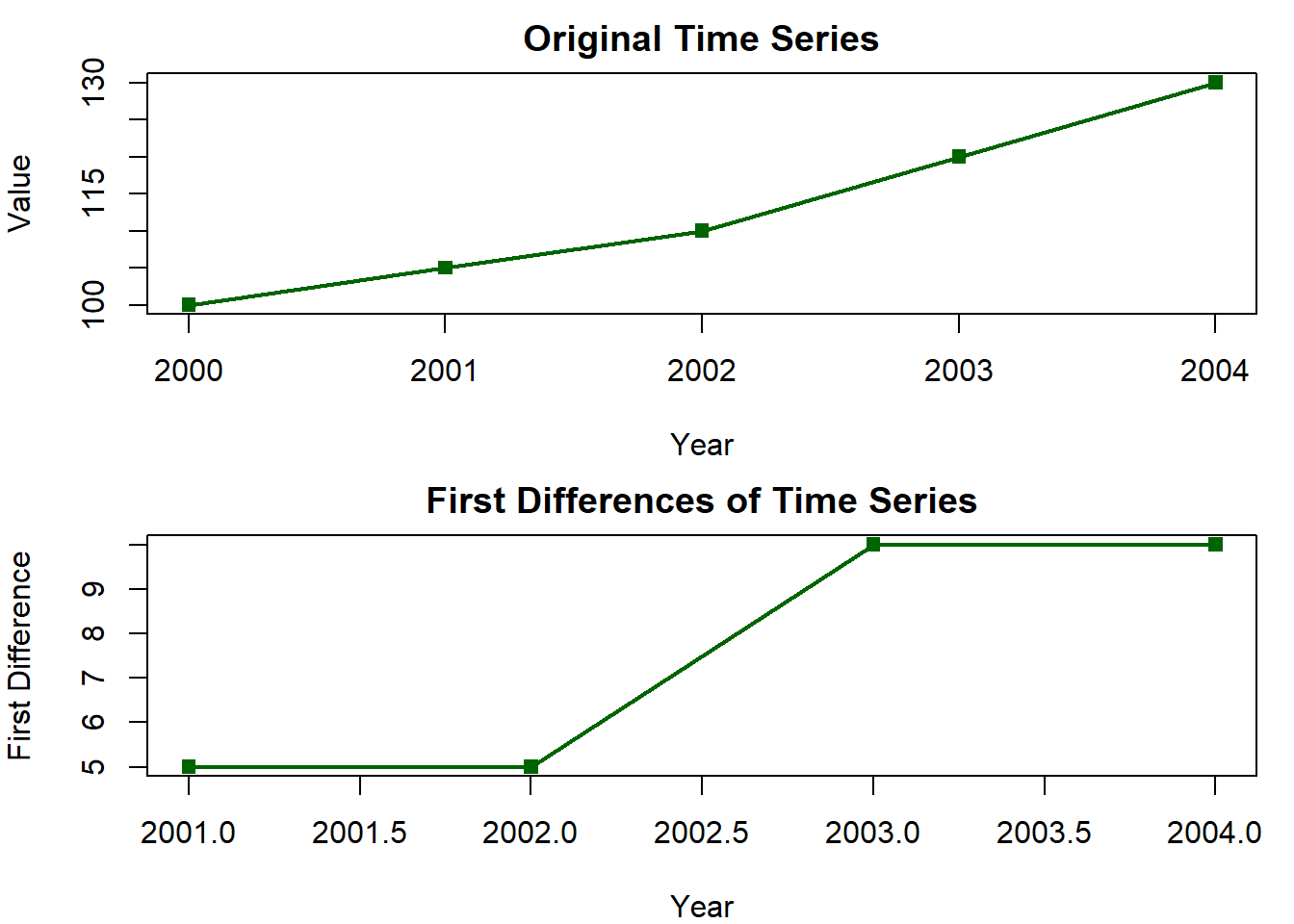
Example with a trending time series:

# Create a time series
ts_data <- ts(c(100, 105, 110, 120, 130), start = 2000)

# Calculate differences
diff_ts <- diff(ts_data)
print(diff_ts)

Time Series:
Start = 2001 
End = 2004 
Frequency = 1 
[1]  5  5 10 10

# Output: 5 5 10 10

# Plot the time series and its differences
par(mfrow = c(2, 1), mar = c(4, 4, 2, 1))

# Original time series
plot(ts_data, type = "o", col = "darkgreen", lwd = 2, pch = 15,
     xlab = "Year", ylab = "Value",
     main = "Original Time Series")

# Differenced time series
plot(diff_ts, type = "o", col = "darkgreen", lwd = 2, pch = 15,
     xlab = "Year", ylab = "First Difference",
     main = "First Differences of Time Series")

# Reset plotting layout
par(mfrow = c(1, 1))

Using the lag Parameter

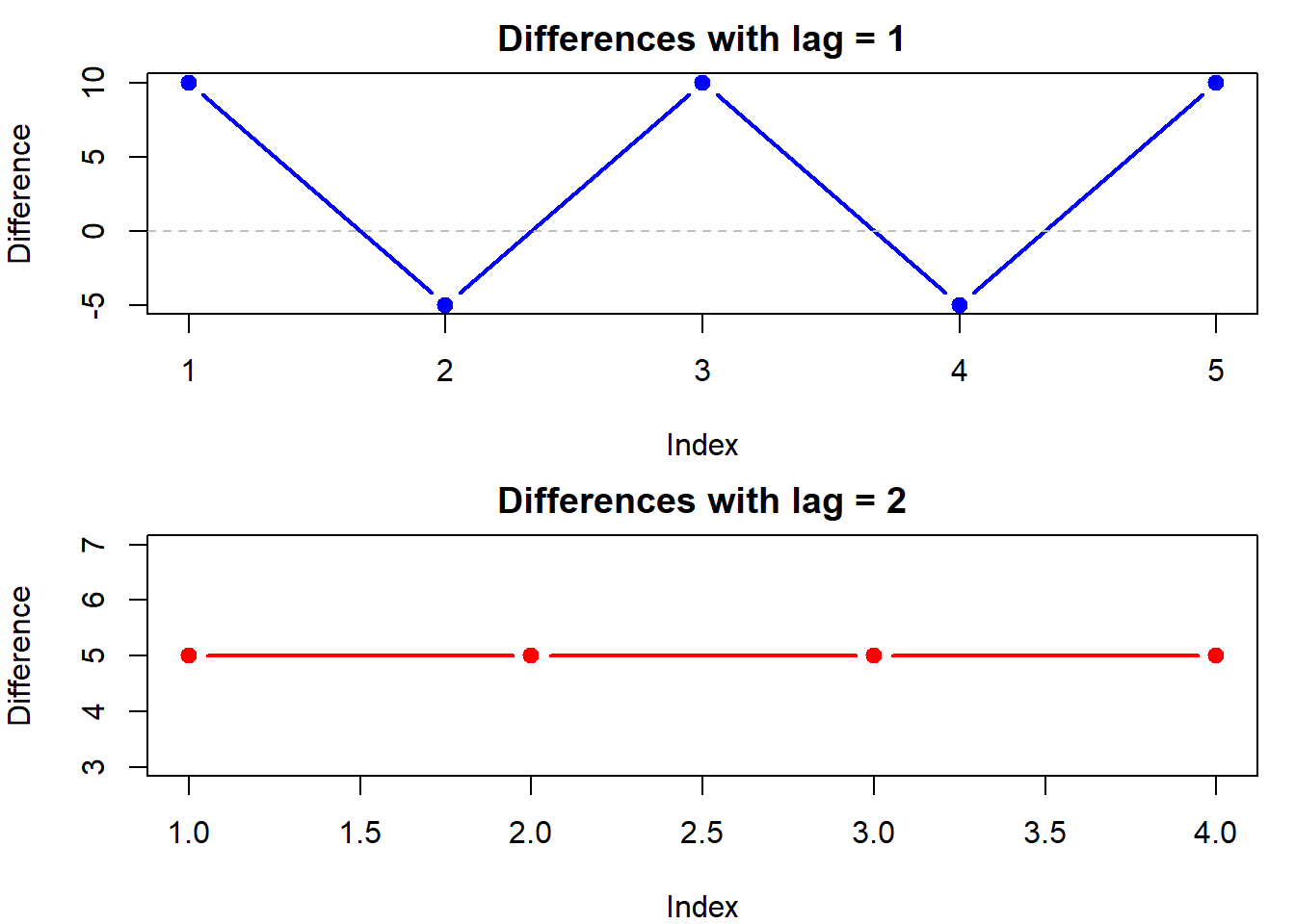
The lag parameter controls how many positions apart the values should be when calculating differences. This is useful for seasonal data or when you want to compare values at specific intervals.

# Create seasonal data
seasonal_data <- c(10, 20, 15, 25, 20, 30)

# Calculate differences with lag=1 and lag=2
diff1 <- diff(seasonal_data, lag = 1)
diff2 <- diff(seasonal_data, lag = 2)

# Plot differences with different lags
par(mfrow = c(2, 1), mar = c(4, 4, 2, 1))

# Lag 1 differences
plot(diff1, type = "b", col = "blue", pch = 19, lwd = 2,
     xlab = "Index", ylab = "Difference",
     main = "Differences with lag = 1")
abline(h = 0, lty = 2, col = "gray")  # Add a reference line at y=0

# Lag 2 differences
plot(diff2, type = "b", col = "red", pch = 19, lwd = 2,
     xlab = "Index", ylab = "Difference",
     main = "Differences with lag = 2")
abline(h = 0, lty = 2, col = "gray")  # Add a reference line at y=0

# Reset plotting layout
par(mfrow = c(1, 1))

With lag = 2, each value is compared to the value from two positions earlier: - For lag=1: 20-10, 15-20, 25-15, 20-25, 30-20 - For lag=2: 15-10, 25-20, 20-15, 30-25

Multiple Differences

You can apply differencing multiple times by setting the differences parameter. This is useful for achieving stationarity in time series with strong trends.

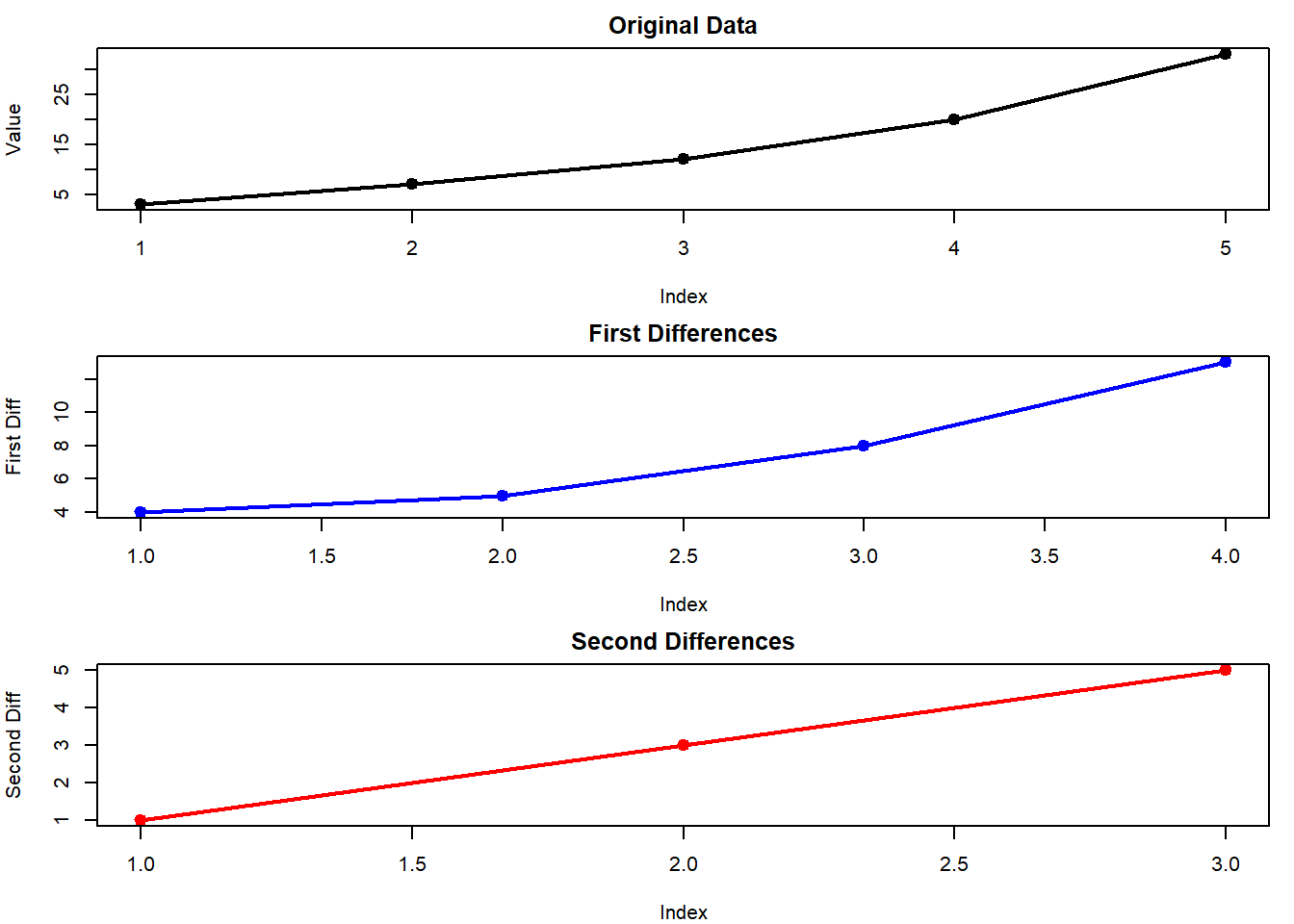
# Create a vector with quadratic growth
vec <- c(3, 7, 12, 20, 33)

# Calculate first and second differences
diff1 <- diff(vec, differences = 1)  # First difference
diff2 <- diff(vec, differences = 2)  # Second difference

print(diff1)  # Output: 4 5 8 13

[1]  4  5  8 13

print(diff2)  # Output: 1 3 5

[1] 1 3 5

# Plot original data and differences
par(mfrow = c(3, 1), mar = c(4, 4, 2, 1))

# Original data
plot(vec, type = "o", col = "black", pch = 19, lwd = 2,
     xlab = "Index", ylab = "Value",
     main = "Original Data")

# First difference
plot(diff1, type = "o", col = "blue", pch = 19, lwd = 2,
     xlab = "Index", ylab = "First Diff",
     main = "First Differences")

# Second difference
plot(diff2, type = "o", col = "red", pch = 19, lwd = 2,
     xlab = "Index", ylab = "Second Diff",
     main = "Second Differences")

# Reset plotting layout
par(mfrow = c(1, 1))

The second difference calculates the differences of the differences: - First differences: 4, 5, 8, 13 - Second differences (differences of differences): 1, 3, 5

Financial Applications

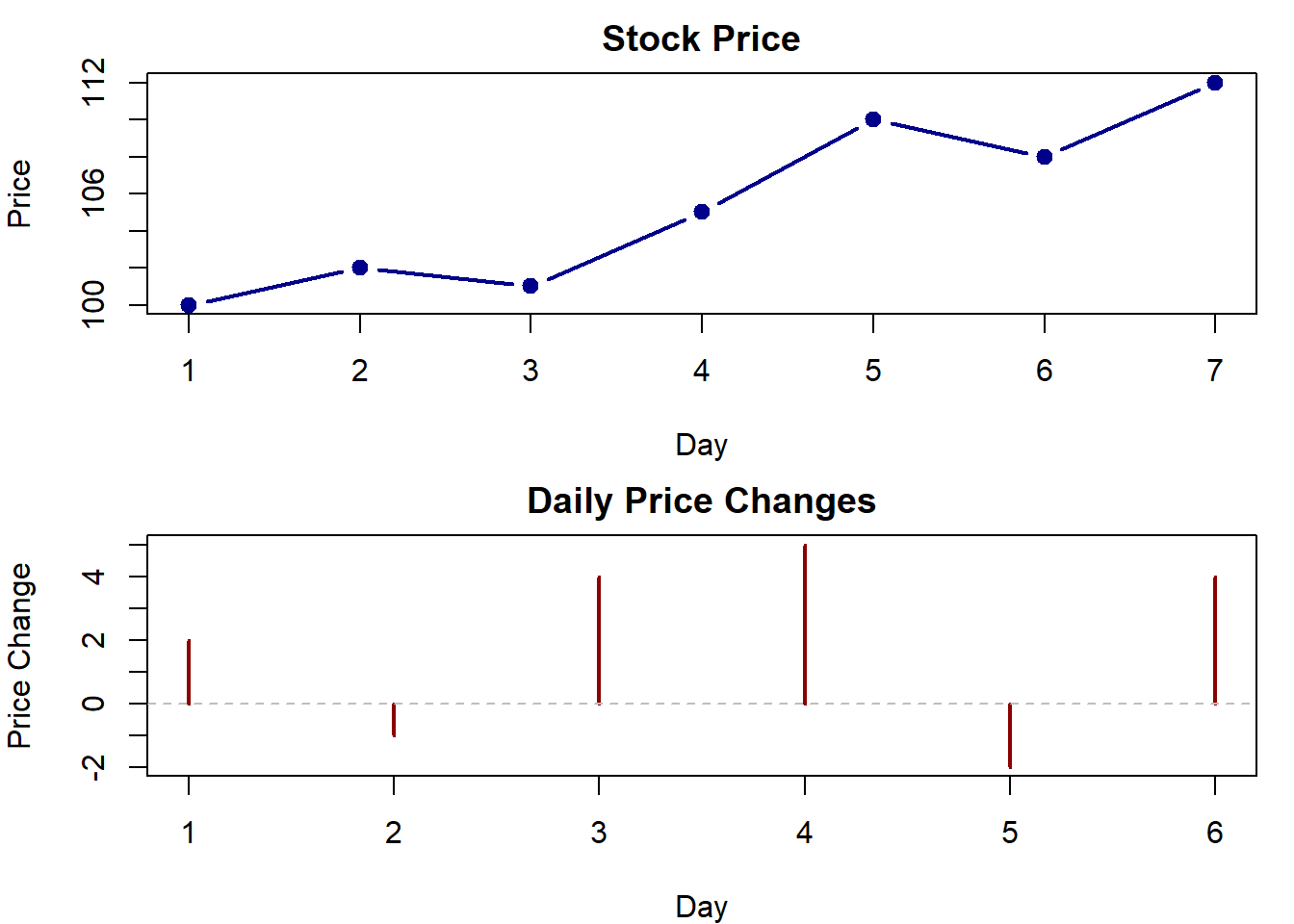
In finance, diff() is commonly used to calculate returns from price data:

# Create price data
prices <- c(100, 102, 101, 105, 110, 108, 112)

# Calculate price changes
returns <- diff(prices)
print(returns)  # Output: 2 -1 4 5 -2 4

[1]  2 -1  4  5 -2  4

# Plot prices and returns
par(mfrow = c(2, 1), mar = c(4, 4, 2, 1))

# Plot prices
plot(prices, type = "b", col = "darkblue", pch = 19, lwd = 2,
     xlab = "Day", ylab = "Price",
     main = "Stock Price")

# Plot returns
plot(returns, type = "h", col = "darkred", lwd = 2,
     xlab = "Day", ylab = "Price Change",
     main = "Daily Price Changes")
abline(h = 0, lty = 2, col = "gray")  # Reference line at y=0

# Reset plotting layout
par(mfrow = c(1, 1))

Common Pitfalls and Edge Cases

1. Output Length Is Shorter

The diff() function always returns a vector that is shorter than the input. For a vector of length n, applying diff() once gives a result of length n-1.

x <- c(10, 15, 20, 18, 25)
cat("Original vector length:", length(x), "\n")

Original vector length: 5

cat("Differenced vector length:", length(diff(x)), "\n")

Differenced vector length: 4

# Output:
# Original vector length: 5
# Differenced vector length: 4

2. Handling Missing Values (NA)

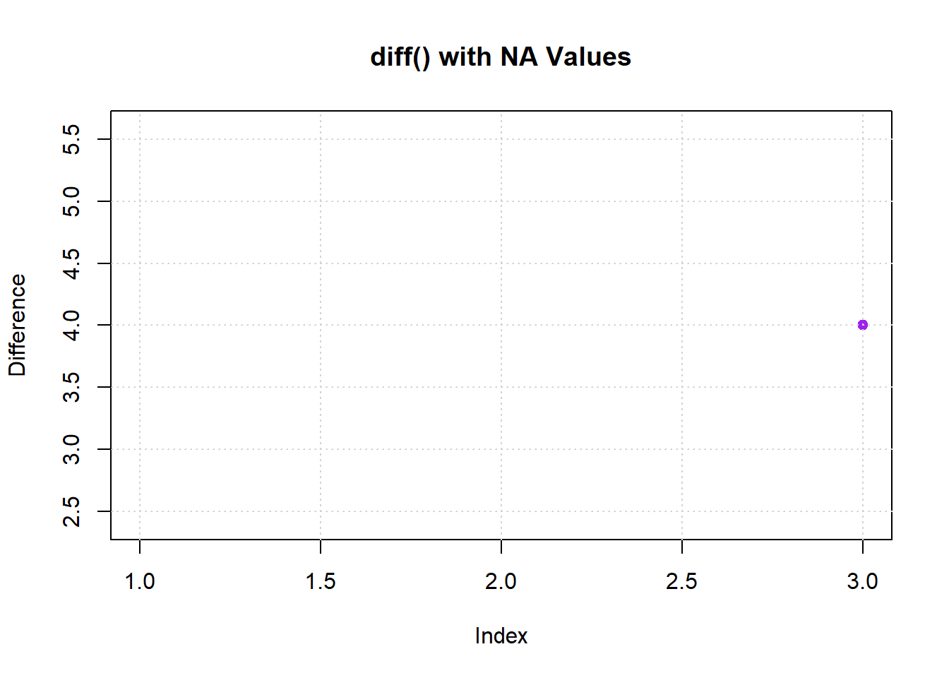
The diff() function propagates NA values. If any element in a pair contains NA, the result for that position will be NA.

# Create vector with NA values
x_na <- c(1, NA, 3, 7)
diff_na <- diff(x_na)
print(diff_na)  # Output: NA NA 4

[1] NA NA  4

# Plot to visualize NA handling
plot(diff_na, type = "o", col = "purple", pch = 19, 
     xlab = "Index", ylab = "Difference",
     main = "diff() with NA Values")
grid()  # Add grid lines for better readability

Here’s how NA values affect the results: - diff(c(1, NA)) = NA - diff(c(NA, 3)) = NA - diff(c(3, 7)) = 4

3. Empty Results

If your input is too short compared to the lag parameter, you might get an empty result:

short_vec <- c(2, 4, 6)
result <- diff(short_vec, lag = 3)
print(result)  # Returns an empty vector

numeric(0)

Best Practices

Check output length: Remember that the output will be shorter than input
Handle NA values: Clean your data before using diff() or handle NAs in the results
Align with original data: If you need to plot or compare with original data, you might need to add NA values to maintain alignment
Verify lag value: Make sure your lag parameter makes sense for your data’s pattern

Quick Summary

diff() calculates the differences between consecutive elements
Basic syntax: diff(x, lag = 1, differences = 1)
Works with vectors, data frames, and time series
Output is always shorter than input by lag × differences
Useful for trend removal, calculating returns, and finding patterns in data
Base R plotting functions like plot() with appropriate parameters provide clear visualization of differences

With the diff() function and base R plotting, you can easily track and visualize changes in your data, remove trends, and prepare data for further analysis.

References

The following references provide additional information about using the diff() function in R and time series analysis:

R Cookbook, 2nd Edition. (n.d.). Time Series Analysis. RC2E.
R-Bloggers. (2023, June). Mastering the Power of R’s diff() Function: A Programmer’s Guide. R-Bloggers.
Coghlan, A. (n.d.). A Little Book of R for Time Series. ReadTheDocs.

Happy Coding! 🚀

You can connect with me at any one of the below:

Telegram Channel here: https://t.me/steveondata

LinkedIn Network here: https://www.linkedin.com/in/spsanderson/

Mastadon Social here: https://mstdn.social/@stevensanderson

RStats Network here: https://rstats.me/@spsanderson

GitHub Network here: https://github.com/spsanderson

Bluesky Network here: https://bsky.app/profile/spsanderson.com

My Book: Extending Excel with Python and R here: https://packt.link/oTyZJ

You.com Referral Link: https://you.com/join/EHSLDTL6