Introduction

Many times in modeling we want to get the uncertainty in the model, well, bootstrapping to the rescue!

I am going to go over a very simple example on how to use purrr and modelr for this situation. We will use the mtcars dataset.

Functions

The main functions that we are going to showcase are purrr::map() and modelr::bootstrap()

Examples

Let’s get right into it.

library(tidyverse)
library(tidymodels)

df <- mtcars

fit_boots <- df %>% 
  modelr::bootstrap(n = 200, id = 'boot_num') %>%
  group_by(boot_num) %>%
  mutate(fit = map(strap, ~lm(mpg ~ ., data = data.frame(.))))

fit_boots

# A tibble: 200 × 3
# Groups:   boot_num [200]
   strap                boot_num fit   
   <list>               <chr>    <list>
 1 <resample [32 x 11]> 001      <lm>  
 2 <resample [32 x 11]> 002      <lm>  
 3 <resample [32 x 11]> 003      <lm>  
 4 <resample [32 x 11]> 004      <lm>  
 5 <resample [32 x 11]> 005      <lm>  
 6 <resample [32 x 11]> 006      <lm>  
 7 <resample [32 x 11]> 007      <lm>  
 8 <resample [32 x 11]> 008      <lm>  
 9 <resample [32 x 11]> 009      <lm>  
10 <resample [32 x 11]> 010      <lm>  
# … with 190 more rows

Now lets get our parameter estimates.

# get parameters ####
params_boot <- fit_boots %>%
  mutate(tidy_fit = map(fit, tidy)) %>%
  unnest(cols = tidy_fit) %>%
  ungroup()

# get predictions
preds_boot <- fit_boots %>%
  mutate(augment_fit = map(fit, augment)) %>%
  unnest(cols = augment_fit) %>%
  ungroup()

Time to visualize.

library(patchwork)

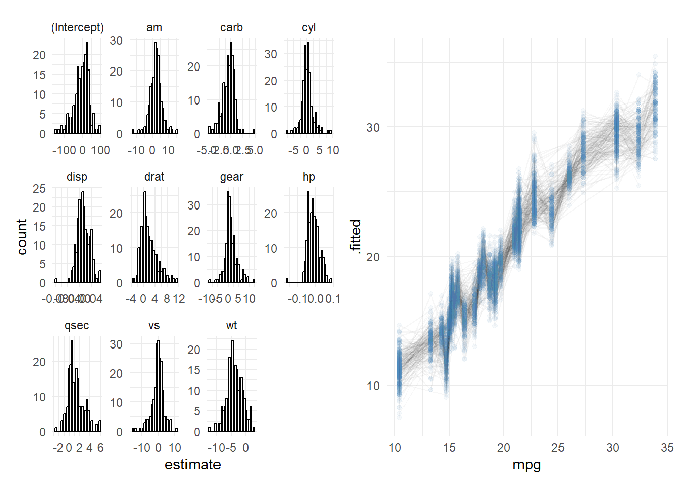
# plot distribution of estimated parameters
p1 <- ggplot(params_boot, aes(estimate)) +
  geom_histogram(col = 'black', fill = 'white') +
  facet_wrap(~ term, scales = 'free') +
  theme_minimal()

# plot points with predictions
p2 <- ggplot() +
  geom_line(aes(mpg, .fitted, group = boot_num), preds_boot, alpha = .03) +
  geom_point(aes(mpg, .fitted), preds_boot, col = 'steelblue', alpha = 0.05) +
  theme_minimal()
  
# plot both
p1 + p2

`stat_bin()` using `bins = 30`. Pick better value with `binwidth`.

Voila!