install.packages("xgboost")Introduction
XGBoost, short for “eXtreme Gradient Boosting,” is a powerful and popular machine learning library that is specifically designed for gradient boosting. It is an open-source library and is available in many programming languages, including R.
Gradient boosting is a technique that combines the predictions of multiple weak models to create a strong, more accurate model. XGBoost is an optimized version of gradient boosting that is designed to run faster and more efficiently than other implementations.
Let’s take a look at a simple example of how to use XGBoost in R. We will use the iris dataset, a well-known dataset that contains 150 observations of iris flowers, each with four features (sepal length, sepal width, petal length, and petal width) and one target variable (the species of iris). Our goal is to train a model to predict the species of an iris flower based on its features.
First, we need to install the “xgboost” package in R:
Next, we load the iris dataset and split it into training and test sets:
data(iris)
set.seed(123)
indices <- sample(1:nrow(iris), 0.8*nrow(iris))
train_data <- iris[indices, 1:4]
train_label <- iris[indices, 5]
test_data <- iris[-indices, 1:4]
test_label <- iris[-indices, 5]
Now we can train our XGBoost model:
library(xgboost)
xgb_model <- xgboost(
  data = train_data,
  label = train_label,
  nrounds = 100,
  objective = "multi:softmax",
  num_class = 3
  )
Here, we specified the training data, labels, number of rounds (iterations) to run, the objective (multiclass classification) and the number of classes.
Finally, we can use the trained model to make predictions on the test set:
predictions <- predict(xgb_model, test_data)We can also evaluate the performance of our model by comparing the predicted labels to the true labels using metrics such as accuracy:
accuracy <- mean(predictions == test_label)In this example, we used XGBoost to train a model to predict the species of iris flowers based on their features. We saw that XGBoost is a powerful and efficient library for gradient boosting, and it can be easily integrated into a R script.
Keep in mind that this is a simple example, and in real-world scenarios, more preprocessing and parameter tuning is necessary to achieve optimal performance. Also, the dataset is small, and the number of rounds used is also small, which is not ideal for real-world scenarios. But this example shows the basic usage of XGBoost in R.
Ok, so, what’s the point? Is there a possibly easier way to do this…yes! You can use the boilerplace function hai_auto_xgboost() and it’s data prep helper hai_xgboost_data_prepper() from the {healthyR.ai} library. Let’s see how that works.
Function
Here is the data prepper function and it’s arguments.
hai_xgboost_data_prepper(.data, .recipe_formula).data- The data that you are passing to the function. Can be any type of data that is accepted by the data parameter of the recipes::reciep() function..recipe_formula- The formula that is going to be passed. For example if you are using the diamonds data then the formula would most likely be something likeprice ~.
Here is the boilerplate function
hai_auto_xgboost(
  .data,
  .rec_obj,
  .splits_obj = NULL,
  .rsamp_obj = NULL,
  .tune = TRUE,
  .grid_size = 10,
  .num_cores = 1,
  .best_metric = "f_meas",
  .model_type = "classification"
)
Here are it’s arguments.
.data- The data being passed to the function. The time-series object..rec_obj- This is the recipe object you want to use. You can usehai_xgboost_data_prepper()an automatic recipe_object..splits_obj- NULL is the default, when NULL then one will be created..rsamp_obj- NULL is the default, when NULL then one will be created. It will default to creating anrsample::mc_cv()object..tune- Default is TRUE, this will create a tuning grid and tuned workflow.grid_size- Default is 10.num_cores- Default is 1.best_metric- Default is “f_meas”. You can choose a metric depending on the model_type used. If regression then seehai_default_regression_metric_set(), if classification then seehai_default_classification_metric_set()..model_type- Default is classification, can also be regression.
Example
Let’s take a look at an example and it’s output. This is using {parsnip} under the hood.
library(healthyR.ai)

data <- iris

rec_obj <- hai_xgboost_data_prepper(data, Species ~ .)

auto_xgb <- hai_auto_xgboost(
  .data = data,
  .rec_obj = rec_obj,
  .best_metric = "f_meas",
  .num_cores = 1
)
There are three main outputs to this function, which are:
recipe_infomodel_infotuned_info
Let’s take a look at each. First the recipe_info
auto_xgb$recipe_info

Recipe

Inputs:

      role #variables
   outcome          1
 predictor          4

Operations:

Factor variables from tidyselect::vars_select_helpers$where(is.charac...
Novel factor level assignment for recipes::all_nominal_predictors()
Dummy variables from recipes::all_nominal_predictors()
Zero variance filter on recipes::all_predictors()
Now the model_info
auto_xgb$model_info

$model_spec
Boosted Tree Model Specification (classification)

Main Arguments:
  trees = tune::tune()
  min_n = tune::tune()
  tree_depth = tune::tune()
  learn_rate = tune::tune()
  loss_reduction = tune::tune()
  sample_size = tune::tune()

Computational engine: xgboost


$wflw
══ Workflow ════════════════════════════════════════════════════════════════════
Preprocessor: Recipe
Model: boost_tree()

── Preprocessor ────────────────────────────────────────────────────────────────
4 Recipe Steps

• step_string2factor()
• step_novel()
• step_dummy()
• step_zv()

── Model ───────────────────────────────────────────────────────────────────────
Boosted Tree Model Specification (classification)

Main Arguments:
  trees = tune::tune()
  min_n = tune::tune()
  tree_depth = tune::tune()
  learn_rate = tune::tune()
  loss_reduction = tune::tune()
  sample_size = tune::tune()

Computational engine: xgboost


$fitted_wflw
══ Workflow [trained] ══════════════════════════════════════════════════════════
Preprocessor: Recipe
Model: boost_tree()

── Preprocessor ────────────────────────────────────────────────────────────────
4 Recipe Steps

• step_string2factor()
• step_novel()
• step_dummy()
• step_zv()

── Model ───────────────────────────────────────────────────────────────────────
##### xgb.Booster
raw: 2.5 Mb
call:
  xgboost::xgb.train(params = list(eta = 0.10962507492329, max_depth = 13L,
    gamma = 0.000498577409120534, colsample_bytree = 1, colsample_bynode = 1,
    min_child_weight = 3L, subsample = 0.594320066112559), data = x$data,
    nrounds = 1240L, watchlist = x$watchlist, verbose = 0, nthread = 1,
    objective = "multi:softprob", num_class = 3L)
params (as set within xgb.train):
  eta = "0.10962507492329", max_depth = "13", gamma = "0.000498577409120534", colsample_bytree = "1", colsample_bynode = "1", min_child_weight = "3", subsample = "0.594320066112559", nthread = "1", objective = "multi:softprob", num_class = "3", validate_parameters = "TRUE"
xgb.attributes:
  niter
callbacks:
  cb.evaluation.log()
# of features: 4
niter: 1240
nfeatures : 4
evaluation_log:
    iter training_mlogloss
       1        0.96929822
       2        0.85785438
---
    1239        0.07815044
    1240        0.07808817

$was_tuned
[1] "tuned"
Now the tuned_info
auto_xgb$tuned_info
$tuning_grid
# A tibble: 10 × 6
trees min_n tree_depth learn_rate loss_reduction sample_size
<int> <int> <int> <dbl> <dbl> <dbl>
1 926 6 2 0.0246 2.21e- 1 0.952
2 1510 25 14 0.00189 1.01e+ 1 0.424
3 1077 29 9 0.195 1.34e- 5 0.319
4 795 32 3 0.00102 1.64e- 3 0.686
5 368 22 4 0.00549 2.97e- 7 0.735
6 1240 3 13 0.110 4.99e- 4 0.594
7 1839 18 5 0.0501 1.67e- 7 0.273
8 139 11 10 0.0153 1.17e- 2 0.483
9 470 40 8 0.0906 6.79e-10 0.168
10 1732 16 11 0.00667 9.19e- 9 0.883
$cv_obj
# Monte Carlo cross-validation (0.75/0.25) with 25 resamples
# A tibble: 25 × 2
splits id
<list> <chr>
1 <split [84/28]> Resample01
2 <split [84/28]> Resample02
3 <split [84/28]> Resample03
4 <split [84/28]> Resample04
5 <split [84/28]> Resample05
6 <split [84/28]> Resample06
7 <split [84/28]> Resample07
8 <split [84/28]> Resample08
9 <split [84/28]> Resample09
10 <split [84/28]> Resample10
# … with 15 more rows
$tuned_results
# Tuning results
# Monte Carlo cross-validation (0.75/0.25) with 25 resamples
# A tibble: 25 × 4
splits id .metrics .notes
<list> <chr> <list> <list>
1 <split [84/28]> Resample01 <tibble [110 × 10]> <tibble [1 × 3]>
2 <split [84/28]> Resample02 <tibble [110 × 10]> <tibble [1 × 3]>
3 <split [84/28]> Resample03 <tibble [110 × 10]> <tibble [1 × 3]>
4 <split [84/28]> Resample04 <tibble [110 × 10]> <tibble [1 × 3]>
5 <split [84/28]> Resample05 <tibble [110 × 10]> <tibble [1 × 3]>
6 <split [84/28]> Resample06 <tibble [110 × 10]> <tibble [1 × 3]>
7 <split [84/28]> Resample07 <tibble [110 × 10]> <tibble [1 × 3]>
8 <split [84/28]> Resample08 <tibble [110 × 10]> <tibble [1 × 3]>
9 <split [84/28]> Resample09 <tibble [110 × 10]> <tibble [1 × 3]>
10 <split [84/28]> Resample10 <tibble [110 × 10]> <tibble [1 × 3]>
# … with 15 more rows
There were issues with some computations:
- Warning(s) x1: While computing multiclass `precision()`, some levels had no pred... - Warning(s) x1: While computing multiclass `precision()`, some levels had no pred... - Warning(s) x1: While computing multiclass `precision()`, some levels had no pred... - Warning(s) x1: While computing multiclass `precision()`, some levels had no pred... - Warning(s) x1: While computing multiclass `precision()`, some levels had no pred... - Warning(s) x1: While computing multiclass `precision()`, some levels had no pred... - Warning(s) x1: While computing multiclass `precision()`, some levels had no pred... - Warning(s) x1: While computing multiclass `precision()`, some levels had no pred... - Warning(s) x1: While computing multiclass `precision()`, some levels had no pred... - Warning(s) x1: While computing multiclass `precision()`, some levels had no pred... - Warning(s) x1: While computing multiclass `precision()`, some levels had no pred... - Warning(s) x1: While computing multiclass `precision()`, some levels had no pred... - Warning(s) x1: While computing multiclass `precision()`, some levels had no pred... - Warning(s) x1: While computing multiclass `precision()`, some levels had no pred... - Warning(s) x1: While computing multiclass `precision()`, some levels had no pred... - Warning(s) x1: While computing multiclass `precision()`, some levels had no pred... - Warning(s) x1: While computing multiclass `precision()`, some levels had no pred... - Warning(s) x1: While computing multiclass `precision()`, some levels had no pred... - Warning(s) x1: While computing multiclass `precision()`, some levels had no pred... - Warning(s) x1: While computing multiclass `precision()`, some levels had no pred... - Warning(s) x1: While computing multiclass `precision()`, some levels had no pred... - Warning(s) x1: While computing multiclass `precision()`, some levels had no pred... - Warning(s) x1: While computing multiclass `precision()`, some levels had no pred... - Warning(s) x1: While computing multiclass `precision()`, some levels had no pred... - Warning(s) x1: While computing multiclass `precision()`, some levels had no pred...
Run `show_notes(.Last.tune.result)` for more information.
$grid_size
[1] 10
$best_metric
[1] "f_meas"
$best_result_set
# A tibble: 1 × 12
trees min_n tree_depth learn_rate loss_r…¹ sampl…² .metric .esti…³ mean n
<int> <int> <int> <dbl> <dbl> <dbl> <chr> <chr> <dbl> <int>
1 1240 3 13 0.110 0.000499 0.594 f_meas macro 0.944 25
# … with 2 more variables: std_err <dbl>, .config <chr>, and abbreviated
# variable names ¹loss_reduction, ²sample_size, ³.estimator
$tuning_grid_plot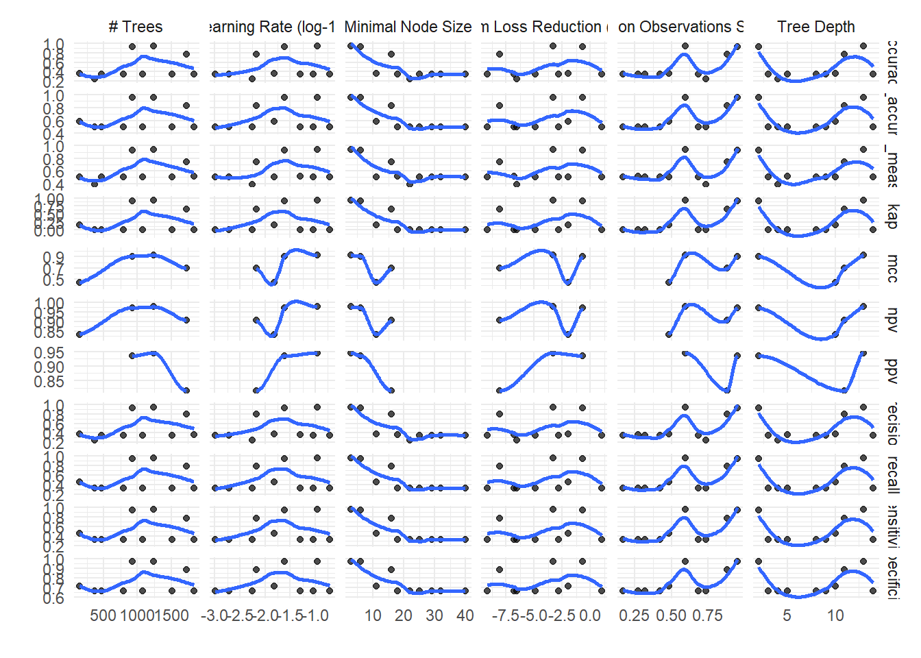
Voila!