Introduction

Transforming data refers to the process of changing the scale or distribution of a variable in order to make it more suitable for analysis. There are many different methods for transforming data, and each has its own specific use case.

Box-Cox: This is a method for transforming data that is positively skewed (i.e., has a long tail to the right) into a more normal distribution. It uses a power transformation to adjust the scale of the data.
Basis Spline: This is a type of non-parametric regression that uses splines (piecewise polynomials) to model the relationship between a dependent variable and one or more independent variables.
Log: This is a method for transforming data that is positively skewed (i.e., has a long tail to the right) into a more normal distribution. It uses the logarithm function to adjust the scale of the data.
Logit: This is a method for transforming binary data (i.e., data with only two possible values) into a continuous scale. It uses the logistic function to adjust the scale of the data.
Natural Spline: This is a type of non-parametric regression that uses splines (piecewise polynomials) to model the relationship between a dependent variable and one or more independent variables, where the splines are chosen to be as smooth as possible.
Rectified Linear Unit (ReLU): This is a type of activation function used in artificial neural networks. It is used to introduce non-linearity in the output of a neuron.
Square Root: This is a method for transforming data that is positively skewed (i.e., has a long tail to the right) into a more normal distribution. It uses the square root function to adjust the scale of the data.
Yeo-Johnson: This is a power transformation that works well for data that is positively or negatively skewed. It is a generalization of the Box-Cox transformation and handles zero and negative data.

The R library {healthyR.ai} provides a function called hai_data_transform() that allows users to easily apply any of these transforms to their data. The function takes in the data and the type of transformation as arguments, and returns the transformed data. This makes it easy for users to experiment with different transformations and see which one works best for their data.

Function

Let’s take a look at the full function call.

hai_data_transform(
  .recipe_object = NULL,
  ...,
  .type_of_scale = "log",
  .bc_limits = c(-5, 5),
  .bc_num_unique = 5,
  .bs_deg_free = NULL,
  .bs_degree = 3,
  .log_base = exp(1),
  .log_offset = 0,
  .logit_offset = 0,
  .ns_deg_free = 2,
  .rel_shift = 0,
  .rel_reverse = FALSE,
  .rel_smooth = FALSE,
  .yj_limits = c(-5, 5),
  .yj_num_unique = 5
)

Now let’s go over the arguments to the parameters.

.recipe_object - The data that you want to process
... - One or more selector functions to choose variables to be imputed. When used with imp_vars, these dots indicate which variables are used to predict the missing data in each variable. See selections() for more details
.type_of_scale - This is a quoted argument and can be one of the following:
- “boxcox”
- “bs”
- “log”
- “logit”
- “ns”
- “relu”
- “sqrt”
- “yeojohnson
.bc_limits - A length 2 numeric vector defining the range to compute the transformation parameter lambda.
.bc_num_unique - An integer to specify minimum required unique values to evaluate for a transformation
.bs_deg_free - The degrees of freedom for the spline. As the degrees of freedom for a spline increase, more flexible and complex curves can be generated. When a single degree of freedom is used, the result is a rescaled version of the original data.
.bs_degree - Degree of polynomial spline (integer).
.log_base - A numeric value for the base.
.log_offset - An optional value to add to the data prior to logging (to avoid log(0))
.logit_offset - A numeric value to modify values of the columns that are either one or zero. They are modifed to be x - offset or offset respectively.
.ns_deg_free - The degrees of freedom for the natural spline. As the degrees of freedom for a natural spline increase, more flexible and complex curves can be generated. When a single degree of freedom is used, the result is a rescaled version of the original data.
.rel_shift - A numeric value dictating a translation to apply to the data.
.rel_reverse - A logical to indicate if the left hinge should be used as opposed to the right hinge.
.rel_smooth - A logical indicating if hte softplus function, a smooth approximation to the rectified linear transformation, should be used.
.yj_limits - A length 2 numeric vector defining the range to compute the transformation parameter lambda.
.yj_num_unique - An integer where data that have less possible values will not be evaluated for a transformation.

Examples

Let’s look over some examples. For an example data set we are going to pick on the mtcars data set as the histogram will prove to be skewed which makes it a good candidate to test these transformations on.

install.packages("healthyR.ai")

Now that we have {healthyR.ai} installed we can get to work. It does use the {recipes} package underneath so you will need to have that installed as well. Let’s look at the histogram of mtcars now.

mpg_vec <- mtcars$mpg

hist(mpg_vec)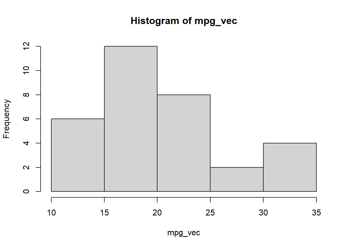

plot(density(mpg_vec))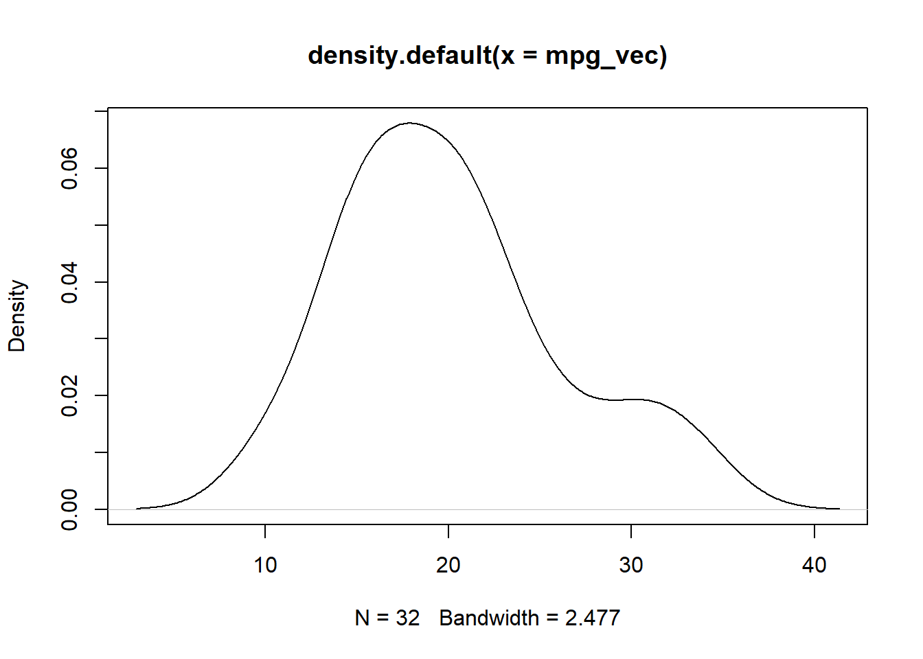

First up, Box-Cox

library(healthyR.ai)
library(recipes)

ro <- recipe(mpg ~ wt, data = mtcars)

boxcox_vec <- hai_data_transform(
  .recipe_object = ro,
  mpg,
  .type_of_scale = "boxcox"
)$scale_rec_obj %>%
  get_juiced_data() %>%
  pull(mpg)

plot(density(boxcox_vec))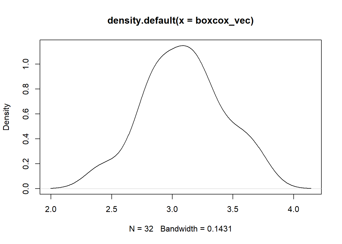

Basis Spline

bs_vec <- hai_data_transform(
  .recipe_object = ro,
  mpg,
  .type_of_scale = "bs"
)$scale_rec_obj %>%
  get_juiced_data()

plot(density(bs_vec$mpg_bs_1))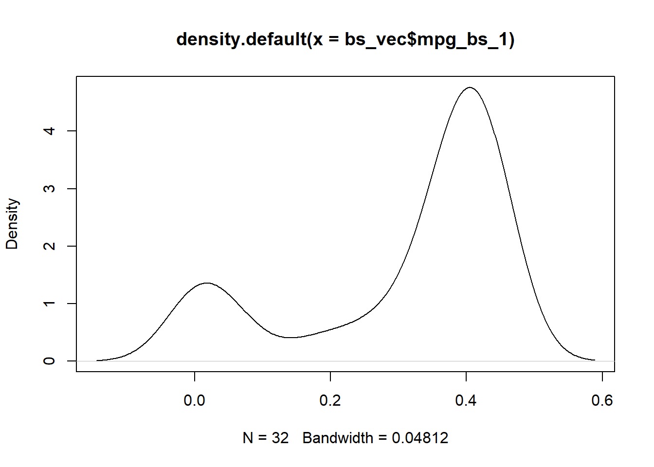

plot(density(bs_vec$mpg_bs_2))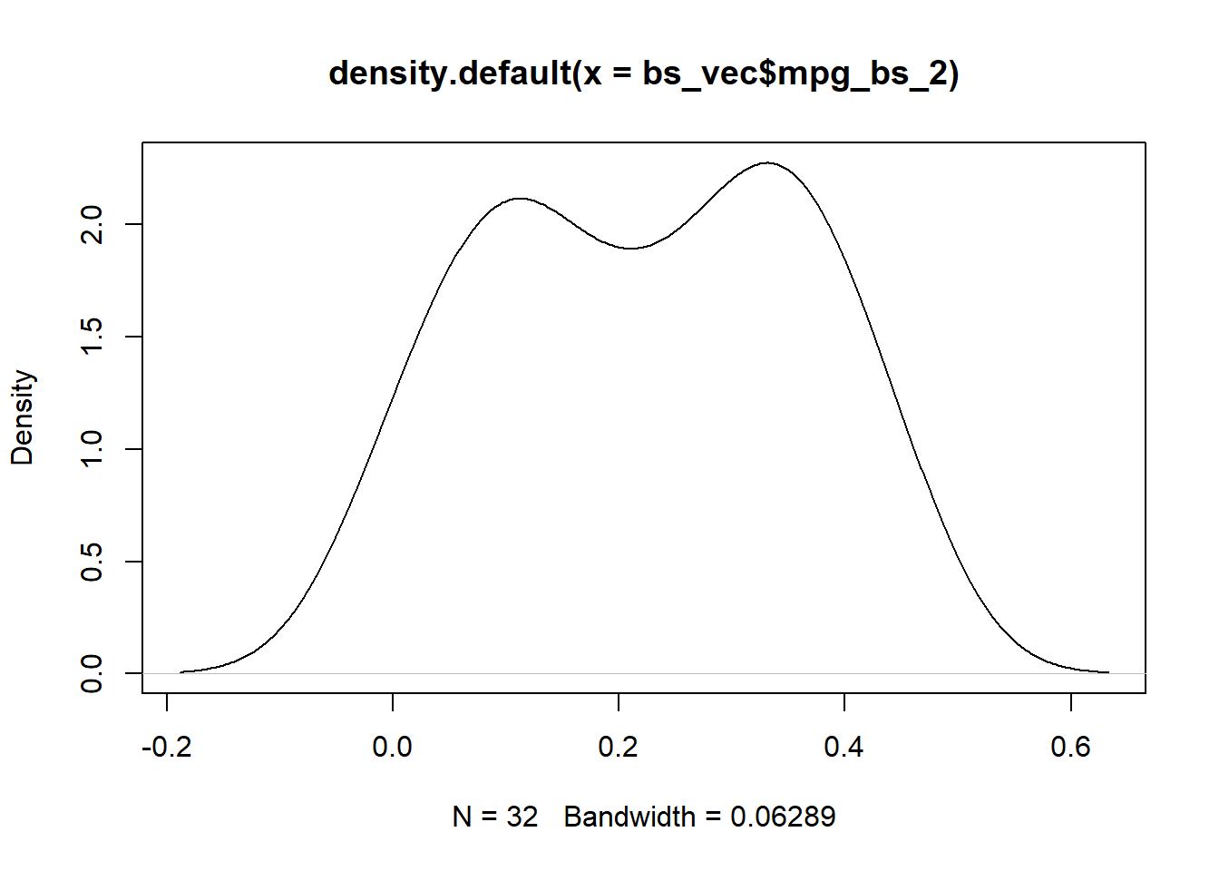

plot(density(bs_vec$mpg_bs_3))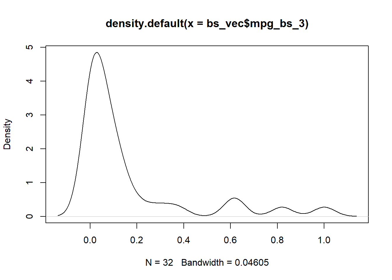

Log

log_vec <- hai_data_transform(
  .recipe_object = ro,
  mpg,
  .type_of_scale = "log"
)$scale_rec_obj %>%
  get_juiced_data() %>%
  pull(mpg)

plot(density(log_vec))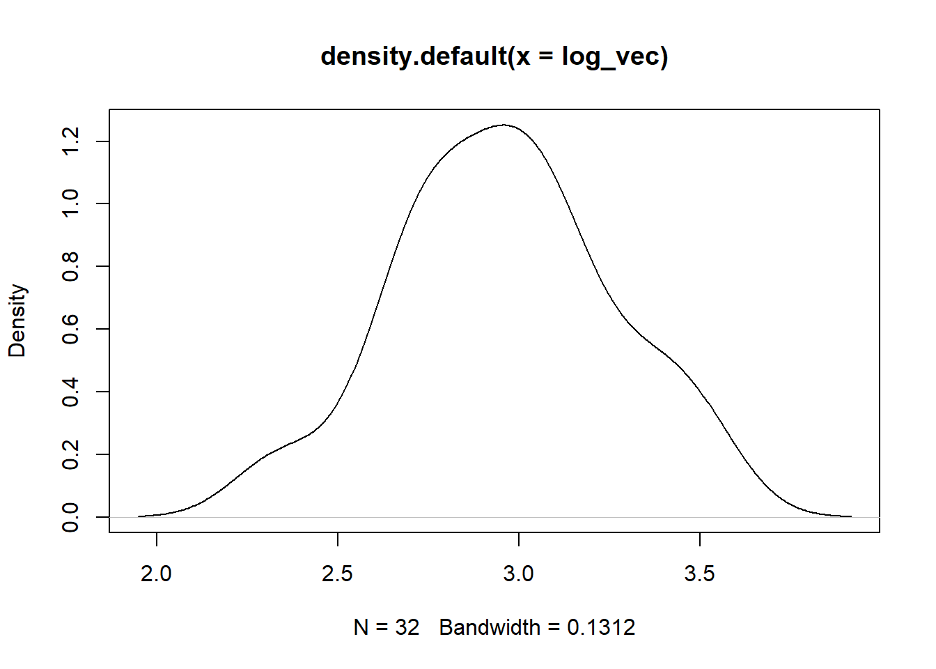

Yeo-Johnson

yj_vec <- hai_data_transform(
  .recipe_object = ro,
  mpg,
  .type_of_scale = "yeojohnson"
)$scale_rec_obj %>%
  get_juiced_data() %>%
  pull(mpg)

plot(density(yj_vec))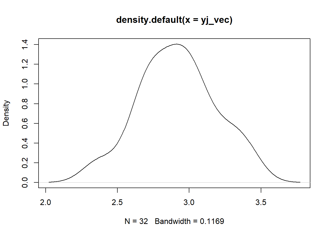

Voila!