Introduction

Shiny is an R package that allows you to create interactive web applications from R code. In this blog post, we’ll explore the different components of a Shiny application and show how they work together to create an interactive data visualization app. This is a part 2 with a small enhancement.

The App

Our Shiny app will generate density plots for different statistical distributions based on user input. The user will be able to select a distribution, set the number of simulations, and choose the plot type from a dropdown menu. The app will also display a table of data generated by the selected distribution.

Here’s a preview of what the app will look like: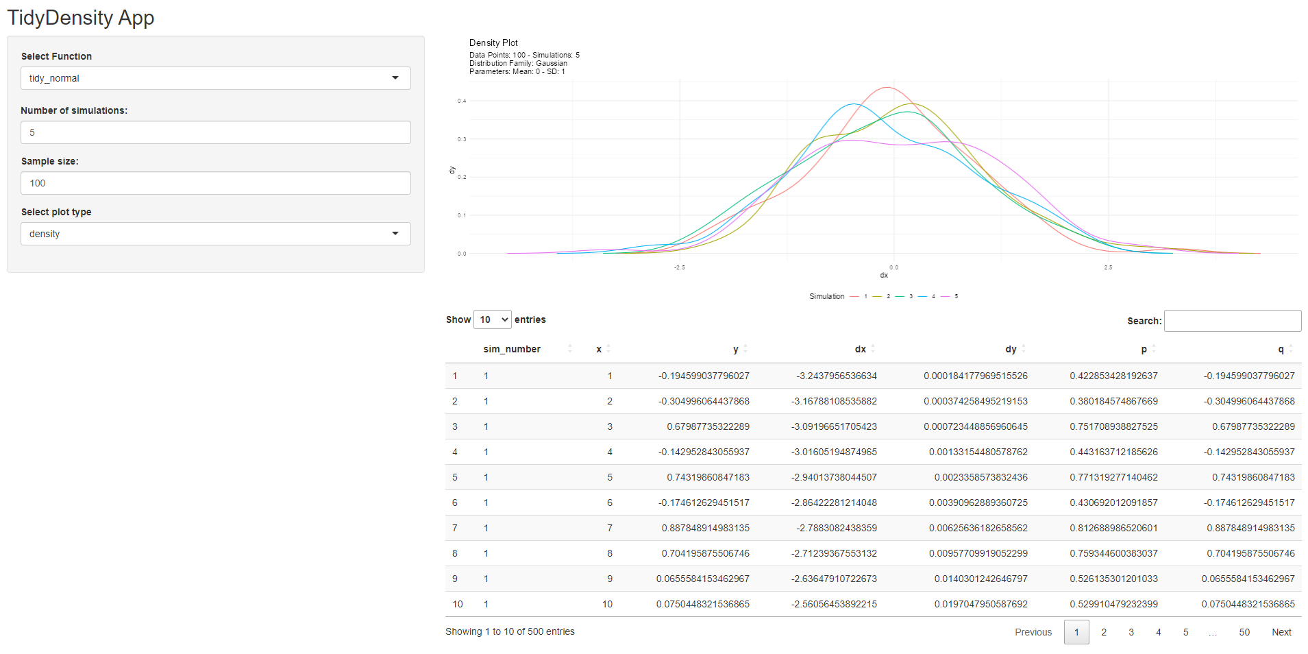

The UI

The user interface (UI) is the visual part of the app that the user interacts with. In our app, the UI is defined using the fluidPage() function from the shiny package. It consists of a title panel, a sidebar layout, and a main panel.

library(shiny)
library(TidyDensity)
library(tidyverse)
library(DT)

# Define UI
ui <- fluidPage(
  titlePanel("TidyDensity App"),
  sidebarLayout(
    sidebarPanel(
      selectInput(inputId = "functions",
                  label = "Select Function",
                  choices = c(
                    "tidy_normal", 
                    "tidy_bernoulli", 
                    "tidy_beta", 
                    "tidy_gamma"
                  )
      ),
      numericInput(inputId = "num_sims",
                   label = "Number of simulations:",
                   value = 1,
                   min = 1,
                   max = 15),
      numericInput(inputId = "n",
                   label = "Sample size:",
                   value = 50,
                   min = 30,
                   max = 200),
      selectInput(inputId = "plot_type",
                  label = "Select plot type",
                  choices = c(
                    "density",
                    "quantile",
                    "probability",
                    "qq",
                    "mcmc"
                  )
      )
    ),
    mainPanel(
      plotOutput("density_plot"),
      DT::dataTableOutput("data_table")
    )
  )
)

The title panel displays the app name, while the sidebar layout contains the input controls for the user. In this case, we have four input elements:

selectInput() allows the user to choose a statistical distribution to generate data from.
numericInput() allows the user to set the number of simulations.
Another numericInput() allows the user to set the sample size.
selectInput() allows the user to choose the type of plot to display.

The main panel contains the output elements for the app, in this case a plot and a table.

The Server

The server is the backend of the app that handles the logic and generates the output based on user input. In our app, the server is defined using the server() function from the shiny package.

# Define server
server <- function(input, output) {
  
  # Create reactive data
  data <- reactive({
    # Call selected function with user input
    match.fun(input$functions)(.num_sims = input$num_sims, .n = input$n)
  })
  
  # Create density plot
  output$density_plot <- renderPlot({
    # Call autoplot on reactive data
    p <- data() |>
      tidy_autoplot(.plot_type = input$plot_type)
    
    print(p)
  })
  
  # Create data table
  output$data_table <- DT::renderDataTable({
    # Return reactive data as a data table
    DT::datatable(data())
  })
  
}

The server() function takes two arguments, input and output. These arguments allow the server to interact with the user interface.

First, we create a reactive data object data, which takes in the user’s input for the function, number of simulations, and sample size, and passes it to the appropriate function using match.fun().

Next, we create the density_plot output. We use the renderPlot() function to create a reactive plot of the data using the tidy_autoplot() function from the {TidyDensity} package. The tidy_autoplot() function allows the user to choose from several plot types, including density, quantile, probability, qq, and mcmc. We then print the plot using the print() function.

Finally, we create the data_table output using the DT::renderDataTable() function. This output displays the reactive data as a table using the DT::datatable() function.

The Shiny App

Finally, we run the Shiny app using the shinyApp() function, which takes the ui and server functions as arguments:

shinyApp(ui = ui, server = server)

This launches the app and displays the user interface. The user can interact with the app by selecting a function, specifying the number of simulations and sample size, and viewing the resulting density plot and data table. The app provides a simple and interactive way to explore the TidyDensity package and its functionality.

Conclusion

Here is the entire app! Steal this code and modify it for yourself, see what you can do!

library(shiny)
library(TidyDensity)
library(tidyverse)
library(DT)

# Define UI
ui <- fluidPage(
  titlePanel("TidyDensity App"),
  sidebarLayout(
    sidebarPanel(
      selectInput(inputId = "functions",
                  label = "Select Function",
                  choices = c(
                    "tidy_normal", 
                    "tidy_bernoulli", 
                    "tidy_beta", 
                    "tidy_gamma"
                  )
      ),
      numericInput(inputId = "num_sims",
                   label = "Number of simulations:",
                   value = 1,
                   min = 1,
                   max = 15),
      numericInput(inputId = "n",
                   label = "Sample size:",
                   value = 50,
                   min = 30,
                   max = 200),
      selectInput(inputId = "plot_type",
                  label = "Select plot type",
                  choices = c(
                    "density",
                    "quantile",
                    "probability",
                    "qq",
                    "mcmc"
                  )
      )
    ),
    mainPanel(
      plotOutput("density_plot"),
      DT::dataTableOutput("data_table")
    )
  )
)

# Define server
server <- function(input, output) {
  
  # Create reactive data
  data <- reactive({
    # Call selected function with user input
    match.fun(input$functions)(.num_sims = input$num_sims, .n = input$n)
  })
  
  # Create density plot
  output$density_plot <- renderPlot({
    # Call autoplot on reactive data
    p <- data() |>
      tidy_autoplot(.plot_type = input$plot_type)
    
    print(p)
  })
  
  # Create data table
  output$data_table <- DT::renderDataTable({
    # Return reactive data as a data table
    DT::datatable(data())
  })
  
}

# Run the app
shinyApp(ui = ui, server = server)

Voila!