Introduction

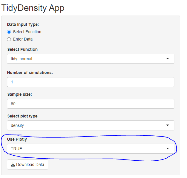
I have been writing about using the {TidyDensity} package with shiny for the last few posts, and this one is the last. This post will go over the app and discuss how to change the output of the graph from a ggplot2 object into a plotly object. So we will end up with something like this in the menu panel:

And here is the difference between the plots, first the ggplot2 plot: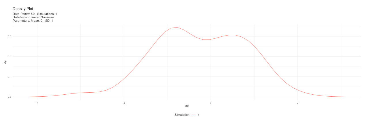

And the plotly_plot: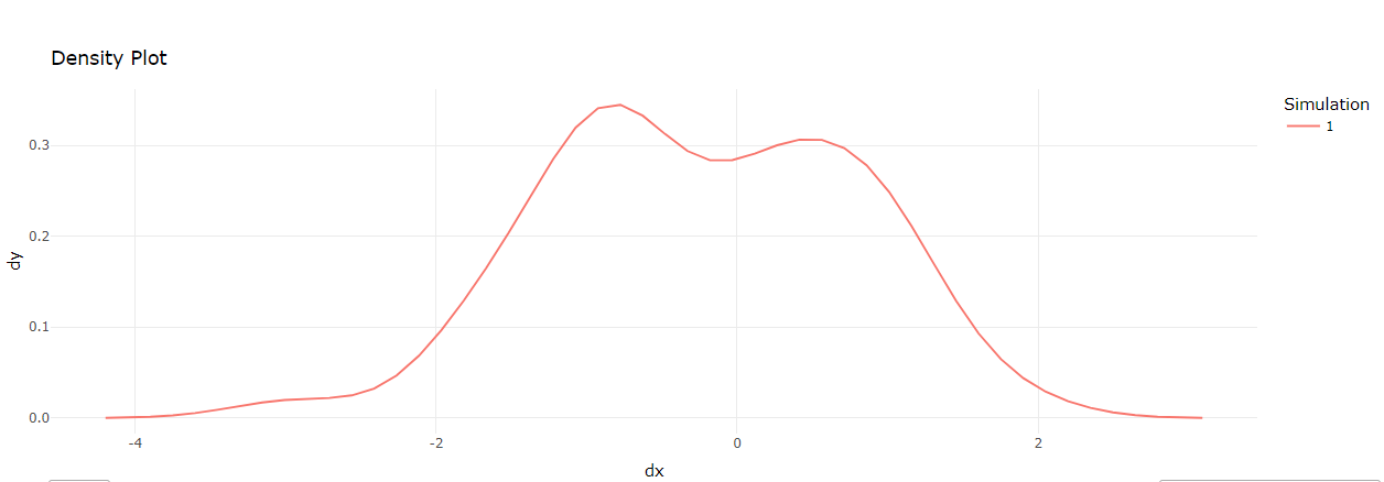

First, the required libraries are loaded: shiny, TidyDensity, tidyverse, DT, and plotly.

library(shiny)
library(TidyDensity)
library(tidyverse)
library(DT)
library(plotly)

UI

The user interface (UI) is defined using the fluidPage() function from the shiny package. The UI consists of a title panel, a sidebar panel, and a main panel. The title panel simply displays the title of the app, while the sidebar panel contains user input elements such as radio buttons, text inputs, and numeric inputs. The main panel displays the plot, data table, and download button.

ui <- fluidPage(
  titlePanel("TidyDensity App"),
  sidebarLayout(
    sidebarPanel(
      # user input elements
    ),
    mainPanel(
      # plot, data table, and download button
    )
  )
)

Next, the server is defined using the server() function from the shiny package. The server is responsible for generating the output based on the user inputs. The first step is to create reactive data using the reactive() function. The reactive data is created based on the user inputs for the distribution function or the entered data. The match.fun() function is used to match the selected function with the corresponding function in the TidyDensity package. The tidy_empirical() function is used if the user entered their own data.

Server

server <- function(input, output) {
  
  # Create reactive data
  data <- reactive({
    # Call selected function with user input or tidy_empirical if user entered data
    if (input$data_input_type == "Enter Data") {
      data <- input$data
      if (is.null(data) || data == "") {
        return(NULL)
      }
      data <- as.numeric(strsplit(data, ",")[[1]])
      tidy_empirical(data)
    } else {
      match.fun(input$functions)(.num_sims = input$num_sims, .n = input$n)
    }
  })

After the reactive data is created, the output is generated. The output consists of the density plot, data table, and download button. The renderPlot() and renderPlotly() functions are used to generate the plot output. The renderDataTable() function is used to generate the data table output. The downloadHandler() function is used to generate the download button.

  # Create density plot
  output$density_plot <- renderPlot({
    # Call autoplot on reactive data
    if (!is.null(data())) {
      p <- data() |>
        tidy_autoplot(.plot_type = input$plot_type)
      
      print(p)
      
      #ifelse(input$plotly_option == "TRUE", ggplotly(p), p)
    }
  })
  
  output$density_plotly <- renderPlotly({
    if (!is.null(data())) {
      p <- data() |>
        tidy_autoplot(.plot_type = input$plot_type)
      
      ggplotly(p)
    }
  })
  
  # Create data table
  output$data_table <- DT::renderDataTable({
    # Return reactive data as a data table
    if (!is.null(data())) {
      DT::datatable(data())

Next, we define the server function, which contains the code that will run in response to user input. We start by creating a reactive data object called data. This object will store the data that will be used to generate the plots and tables in the app.

The data that data stores depends on the user’s input. If the user selects “Enter Data” in the sidebar, then data will be set to a tidy_empirical() object generated from the user-entered data. Otherwise, if the user selects “Select Function”, then data will be set to a tidy_ function object generated using the user’s choices for number of simulations and sample size.

# Define server
server <- function(input, output) {
  
  # Create reactive data
  data <- reactive({
    # Call selected function with user input or tidy_empirical if user entered data
    if (input$data_input_type == "Enter Data") {
      data <- input$data
      if (is.null(data) || data == "") {
        return(NULL)
      }
      data <- as.numeric(strsplit(data, ",")[[1]])
      tidy_empirical(data)
    } else {
      match.fun(input$functions)(.num_sims = input$num_sims, .n = input$n)
    }
  })
  ...
}

The tidy_empirical() function is used to generate a density plot of the empirical distribution of the user-entered data. This function takes the user-entered data as input and returns a tidy data frame that can be used to create a density plot.

The tidy_ functions are used to simulate data from various distributions and generate plots based on that data. These functions take the number of simulations and sample size as input and return a tidy data frame that can be used to create various types of plots.

Next, we define the code for generating the density plot. This code uses the data object that was created earlier to generate a plot. The tidy_autoplot() function is used to generate the plot based on the user’s selected plot type. If the user selects the “Use Plotly” option, then the plot is generated using the ggplotly() function from the plotly package.

 # Create density plot
  output$density_plot <- renderPlot({
    # Call autoplot on reactive data
    if (!is.null(data())) {
      p <- data() |>
        tidy_autoplot(.plot_type = input$plot_type)
      
      print(p)
      
      #ifelse(input$plotly_option == "TRUE", ggplotly(p), p)
    }
  })
  
  output$density_plotly <- renderPlotly({
    if (!is.null(data())) {
      p <- data() |>
        tidy_autoplot(.plot_type = input$plot_type)
      
      ggplotly(p)
    }
  })

The ggplotly() function is used to generate an interactive version of the plot that can be zoomed in and out of and hovered over to see details about specific data points.

Next, we define the code for generating the data table. This code simply displays the data object as a table using the datatable() function from the DT package.

# Create data table
output$data_table <- DT::renderDataTable({
  # Return reactive data as a data table
  if (!is.null(data())) {
    DT::datatable(data())
  }
})

Finally, we define the code for downloading the data as a CSV file. This code uses the downloadHandler() function to generate a file download link that, when clicked, will download the data as a CSV file. The name of the CSV file depends on the user’s input.

  # Download data handler
  output$download_data <- downloadHandler(
    filename = function() {
      if (input$data_input_type == "Enter Data") {
        paste0("tidy_empirical.csv")
      } else {
        paste0(input$functions, ".csv")
      }
    },
    content = function(file) {
      write.csv(data(), file, row.names = FALSE)
    }
  )

Finally, here is the script in it’s entirety, steal it and see what you can come up with!!

library(shiny)
library(TidyDensity)
library(tidyverse)
library(DT)
library(plotly)

# Define UI
ui <- fluidPage(
  titlePanel("TidyDensity App"),
  sidebarLayout(
    sidebarPanel(
      radioButtons(inputId = "data_input_type",
                   label = "Data Input Type:",
                   choices = c("Select Function", "Enter Data"),
                   selected = "Select Function"),
      conditionalPanel(
        condition = "input.data_input_type == 'Enter Data'",
        textInput(inputId = "data",
                  label = "Enter data as a comma-separated list of numeric values")
      ),
      conditionalPanel(
        condition = "input.data_input_type == 'Select Function'",
        selectInput(inputId = "functions",
                    label = "Select Function",
                    choices = c(
                      "tidy_normal", 
                      "tidy_bernoulli", 
                      "tidy_beta", 
                      "tidy_gamma"
                    )
        )
      ),
      numericInput(inputId = "num_sims",
                   label = "Number of simulations:",
                   value = 1,
                   min = 1,
                   max = 15),
      numericInput(inputId = "n",
                   label = "Sample size:",
                   value = 50,
                   min = 30,
                   max = 200),
      selectInput(inputId = "plot_type",
                  label = "Select plot type",
                  choices = c(
                    "density",
                    "quantile",
                    "probability",
                    "qq",
                    "mcmc"
                  )
      ),
      selectInput(inputId = "plotly_option",
                  label = "Use Plotly",
                  choices = c("TRUE", "FALSE"),
                  selected = "FALSE"
      ),
      downloadButton(outputId = "download_data", label = "Download Data")
    ),
    mainPanel(
      conditionalPanel(
        condition = "input.plotly_option == 'TRUE'",
        plotlyOutput("density_plotly")
      ),
      conditionalPanel(
        condition = "input.plotly_option == 'FALSE'",
        plotOutput("density_plot")
      ),
      DT::dataTableOutput("data_table")
    )
  )
)

# Define server
server <- function(input, output) {
  
  # Create reactive data
  data <- reactive({
    # Call selected function with user input or tidy_empirical if user entered data
    if (input$data_input_type == "Enter Data") {
      data <- input$data
      if (is.null(data) || data == "") {
        return(NULL)
      }
      data <- as.numeric(strsplit(data, ",")[[1]])
      tidy_empirical(data)
    } else {
      match.fun(input$functions)(.num_sims = input$num_sims, .n = input$n)
    }
  })
  
  # Create density plot
  output$density_plot <- renderPlot({
    # Call autoplot on reactive data
    if (!is.null(data())) {
      p <- data() |>
        tidy_autoplot(.plot_type = input$plot_type)
      
      print(p)
      
      #ifelse(input$plotly_option == "TRUE", ggplotly(p), p)
    }
  })
  
  output$density_plotly <- renderPlotly({
    if (!is.null(data())) {
      p <- data() |>
        tidy_autoplot(.plot_type = input$plot_type)
      
      ggplotly(p)
    }
  })
  
  # Create data table
  output$data_table <- DT::renderDataTable({
    # Return reactive data as a data table
    if (!is.null(data())) {
      DT::datatable(data())
    }
  })
  
  # Download data handler
  output$download_data <- downloadHandler(
    filename = function() {
      if (input$data_input_type == "Enter Data") {
        paste0("tidy_empirical.csv")
      } else {
        paste0(input$functions, ".csv")
      }
    },
    content = function(file) {
      write.csv(data(), file, row.names = FALSE)
    }
  )
  
}

# Run
shinyApp(ui = ui, server = server)

Voila!