Introduction

Minimal coding ML is not something that is unheard of and is rather prolific, think h2o and pycaret just to name two. There is also no shortage available for R with the h2o interface, and tidyfit. There are also similar low-code workflows in my r package {healthyR.ai}. Today I will specifically go through the workflow for Automatic KNN classification for the Iris data set where we will classify the Species.

Function

Let’s take a look at the two {healthyR.ai} functions that we will be using. First we have the data prepper hai_knn_data_prepper() which will get the data ready for use with the knn algorithm, and then we have the actual auto ml function hai_auto_knn(). Let’s take a look at the function calls.

First hai_knn_data_prepper()

hai_knn_data_prepper(.data, .recipe_formula)

Now let’s look at the arguments to those parameters.

.data - The data that you are passing to the function. Can be any type of data that is accepted by the data parameter of the recipes::reciep() function.
.recipe_formula - The formula that is going to be passed. For example if you are using the iris data then the formula would most likely be something like Species ~ .

Now let’s take a look at the automl function.

hai_auto_knn(
  .data,
  .rec_obj,
  .splits_obj = NULL,
  .rsamp_obj = NULL,
  .tune = TRUE,
  .grid_size = 10,
  .num_cores = 1,
  .best_metric = "rmse",
  .model_type = "regression"
)

Again let’s look at the arguments to the parameters.

.data - The data being passed to the function. The time-series object.
.rec_obj - This is the recipe object you want to use. You can use hai_knn_data_prepper() an automatic recipe_object.
.splits_obj - NULL is the default, when NULL then one will be created.
.rsamp_obj - NULL is the default, when NULL then one will be created. It will default to creating an rsample::mc_cv() object.
.tune - Default is TRUE, this will create a tuning grid and tuned workflow
.grid_size - Default is 10
.num_cores - Default is 1
.best_metric - Default is “rmse”. You can choose a metric depending on the model_type used. If regression then see hai_default_regression_metric_set(), if classification then see hai_default_classification_metric_set().
.model_type - Default is regression, can also be classification.

Example

For this example we are going to use the iris data set where we are going to use the hai_auto_knn() to classify the Species.

library(healthyR.ai)

data <- iris

rec_obj <- hai_knn_data_prepper(data, Species ~ .)

auto_knn <- hai_auto_knn(
  .data = data,
  .rec_obj = rec_obj,
  .best_metric = "f_meas",
  .model_type = "classification",
  .num_cores = 12
)

Now let’s take a look at the complete output of the auto_knn object. The outputs are as follows:

recipe
model specification
workflow
tuned model (grid ect)

Recipe Output

auto_knn$recipe_info

Recipe

Inputs:

      role #variables
   outcome          1
 predictor          4

Operations:

Novel factor level assignment for recipes::all_nominal_predictors()
Dummy variables from recipes::all_nominal_predictors()
Zero variance filter on recipes::all_predictors()
Centering and scaling for recipes::all_numeric()

Model Info

auto_knn$model_info$was_tuned

[1] "tuned"

auto_knn$model_info$model_spec

K-Nearest Neighbor Model Specification (classification)

Main Arguments:
  neighbors = tune::tune()
  weight_func = tune::tune()
  dist_power = tune::tune()

Computational engine: kknn

auto_knn$model_info$wflw

══ Workflow ════════════════════════════════════════════════════════════════════
Preprocessor: Recipe
Model: nearest_neighbor()

── Preprocessor ────────────────────────────────────────────────────────────────
4 Recipe Steps

• step_novel()
• step_dummy()
• step_zv()
• step_normalize()

── Model ───────────────────────────────────────────────────────────────────────
K-Nearest Neighbor Model Specification (classification)

Main Arguments:
  neighbors = tune::tune()
  weight_func = tune::tune()
  dist_power = tune::tune()

Computational engine: kknn

auto_knn$model_info$fitted_wflw

══ Workflow [trained] ══════════════════════════════════════════════════════════
Preprocessor: Recipe
Model: nearest_neighbor()

── Preprocessor ────────────────────────────────────────────────────────────────
4 Recipe Steps

• step_novel()
• step_dummy()
• step_zv()
• step_normalize()

── Model ───────────────────────────────────────────────────────────────────────

Call:
kknn::train.kknn(formula = ..y ~ ., data = data, ks = min_rows(13L,     data, 5), distance = ~1.69935879141092, kernel = ~"rank")

Type of response variable: nominal
Minimal misclassification: 0.03571429
Best kernel: rank
Best k: 13

Tuning Info

auto_knn$tuned_info$tuning_grid

# A tibble: 10 × 3
   neighbors weight_func  dist_power
       <int> <chr>             <dbl>
 1         4 triangular        0.764
 2        11 rectangular       0.219
 3         5 gaussian          1.35 
 4        14 triweight         0.351
 5         5 biweight          1.05 
 6         9 optimal           1.87 
 7         7 cos               0.665
 8        11 inv               1.18 
 9        13 rank              1.70 
10         1 epanechnikov      1.58

auto_knn$tuned_info$cv_obj

# Monte Carlo cross-validation (0.75/0.25) with 25 resamples  
# A tibble: 25 × 2
   splits          id        
   <list>          <chr>     
 1 <split [84/28]> Resample01
 2 <split [84/28]> Resample02
 3 <split [84/28]> Resample03
 4 <split [84/28]> Resample04
 5 <split [84/28]> Resample05
 6 <split [84/28]> Resample06
 7 <split [84/28]> Resample07
 8 <split [84/28]> Resample08
 9 <split [84/28]> Resample09
10 <split [84/28]> Resample10
# … with 15 more rows

auto_knn$tuned_info$tuned_results

# Tuning results
# Monte Carlo cross-validation (0.75/0.25) with 25 resamples  
# A tibble: 25 × 4
   splits          id         .metrics           .notes          
   <list>          <chr>      <list>             <list>          
 1 <split [84/28]> Resample01 <tibble [110 × 7]> <tibble [0 × 3]>
 2 <split [84/28]> Resample02 <tibble [110 × 7]> <tibble [0 × 3]>
 3 <split [84/28]> Resample03 <tibble [110 × 7]> <tibble [0 × 3]>
 4 <split [84/28]> Resample04 <tibble [110 × 7]> <tibble [0 × 3]>
 5 <split [84/28]> Resample05 <tibble [110 × 7]> <tibble [0 × 3]>
 6 <split [84/28]> Resample06 <tibble [110 × 7]> <tibble [0 × 3]>
 7 <split [84/28]> Resample07 <tibble [110 × 7]> <tibble [0 × 3]>
 8 <split [84/28]> Resample08 <tibble [110 × 7]> <tibble [0 × 3]>
 9 <split [84/28]> Resample09 <tibble [110 × 7]> <tibble [0 × 3]>
10 <split [84/28]> Resample10 <tibble [110 × 7]> <tibble [0 × 3]>
# … with 15 more rows

auto_knn$tuned_info$grid_size

[1] 10

auto_knn$tuned_info$best_metric

[1] "f_meas"

auto_knn$tuned_info$best_result_set

# A tibble: 1 × 9
  neighbors weight_func dist_power .metric .estima…¹  mean     n std_err .config
      <int> <chr>            <dbl> <chr>   <chr>     <dbl> <int>   <dbl> <chr>  
1        13 rank              1.70 f_meas  macro     0.957    25 0.00655 Prepro…
# … with abbreviated variable name ¹.estimator

auto_knn$tuned_info$tuning_grid_plot

`geom_smooth()` using method = 'loess' and formula = 'y ~ x'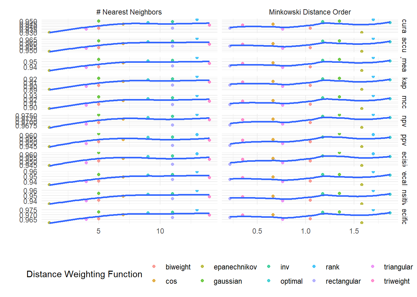

auto_knn$tuned_info$plotly_grid_plot

Voila!

Thank you for reading.