Introduction

Many times in the real world we have a data set which is actually a sample as we typically do not know what the actual population is. This is where bootstrapping tends to come into play. It allows us to get a hold on what the possible parameter values are by taking repeated samples of the data that is available to us.

At it’s core it is a resampling method with replacement where it assigns measures of accuracy to the sample estimates. Here is the Wikipedia Article for bootstrapping.

In this post I am going to go over how to use the bootstrap function set with {TidyDensity}. You can find the pkgdown site with all function references here: TidyDensity

Bootstrapping with TidyDensity

The first thing we will need is a dataset, and for this we are going to pick on the mtcars dataset and more specifically the mpg column. So let’s get to it!

x <- mtcars$mpg

x

 [1] 21.0 21.0 22.8 21.4 18.7 18.1 14.3 24.4 22.8 19.2 17.8 16.4 17.3 15.2 10.4
[16] 10.4 14.7 32.4 30.4 33.9 21.5 15.5 15.2 13.3 19.2 27.3 26.0 30.4 15.8 19.7
[31] 15.0 21.4

We see that x is a numeric vector, which is what we need for these {TidyDensity} functions. The first function that x will be put through is a function called tidy_bootstrap() Let’s take a look at the full function call and parameters of this function.

tidy_bootstrap(
  .x,
  .num_sims = 2000,
  .proportion = 0.8,
  .distribution_type = "continuous"
)

What you see above are the defaults for the function. Now lets go through the parameters.

.x - This is of course the numeric vector that you are passing to the function, in our case right now, it is x which we set to mtcars$mpg
.num_sims - This is how many simulations you want to run of x. This is done with replacement. So this is dictating how many bootstrap samples of x we want to take.
.proportion - How much of the data do you want to sample? The default here is 80%
.distribution_type - What kind of distribution are you sampling from? Is it a continuous or discrete distribution. This is important for plotting.

The function returns a tibble with the bootstrap column as a list object. Lets take a look at tidy_bootstrap(x). We are going to set simulations to 50 instead of the default 2000.

library(TidyDensity)
tb <- tidy_bootstrap(x, .num_sims = 50)

tb

# A tibble: 50 × 2
   sim_number bootstrap_samples
   <fct>      <list>           
 1 1          <dbl [25]>       
 2 2          <dbl [25]>       
 3 3          <dbl [25]>       
 4 4          <dbl [25]>       
 5 5          <dbl [25]>       
 6 6          <dbl [25]>       
 7 7          <dbl [25]>       
 8 8          <dbl [25]>       
 9 9          <dbl [25]>       
10 10         <dbl [25]>       
# … with 40 more rows

The column bootstrap_samples holds the bootstrapped resamples of x at the given .proportion, in this instance, 80%.

From this point we can go straight into use the bootstrap_stat_plot() function if we choose. Under-the-hood it will make use of bootstrap_unnest_tbl(). All this function does is act as a helper to unnest the bootstrap_samples column of the returned tibble from tidy_bootstrap() Let’s take a look below.

tb %>%
  bootstrap_unnest_tbl()

# A tibble: 1,250 × 2
   sim_number     y
   <fct>      <dbl>
 1 1           22.8
 2 1           15.5
 3 1           21.5
 4 1           15  
 5 1           10.4
 6 1           22.8
 7 1           16.4
 8 1           30.4
 9 1           26  
10 1           19.2
# … with 1,240 more rows

Now let’s get into the bootstrap_stat_plot() function of {TidyDensity}

Bootstrap Stat Plot

The function bootstrap_stat_plot() was designed to handle data either from the tidy_bootstrap() or bootstrap_unnest_tbl() functions only. This was to ensure that the right type of data was being passed in and to ensure that the right type of output was guaranteed.

Let’s take a full look at the function call.

bootstrap_stat_plot(
  .data,
  .value,
  .stat = "cmean",
  .show_groups = FALSE,
  .show_ci_labels = TRUE,
  .interactive = FALSE
)

There are a few interesting parameters here, but like before we will go through all of them.

.data - This is the data that gets passed from either tidy_bootstrap() or bootstrap_unnest_tbl()
.value - This is the column from bootstrap_unnest_tbl() that you want to visualize, this is typically y
.stat - There are multiple cumulative stats that will work with this plot. These are all built directly into the {TidyDensity} package. You can find the supported ones that are built into this package at the reference page.
.show_groups - Do you want to show all of the simulation groups TRUE/FALSE
.show_ci_labels - If set to TRUE then the confidence interval labels will be shows on the graph as the final value.
.interactive - Do you want a plotly plot? Who doesn’t?

Now let’s walk though a few examples.

Cumulative Mean

tb %>%
  bootstrap_stat_plot(.value = y)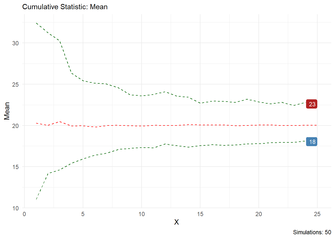

tb %>%
  bootstrap_stat_plot(.value = y, .show_groups = TRUE)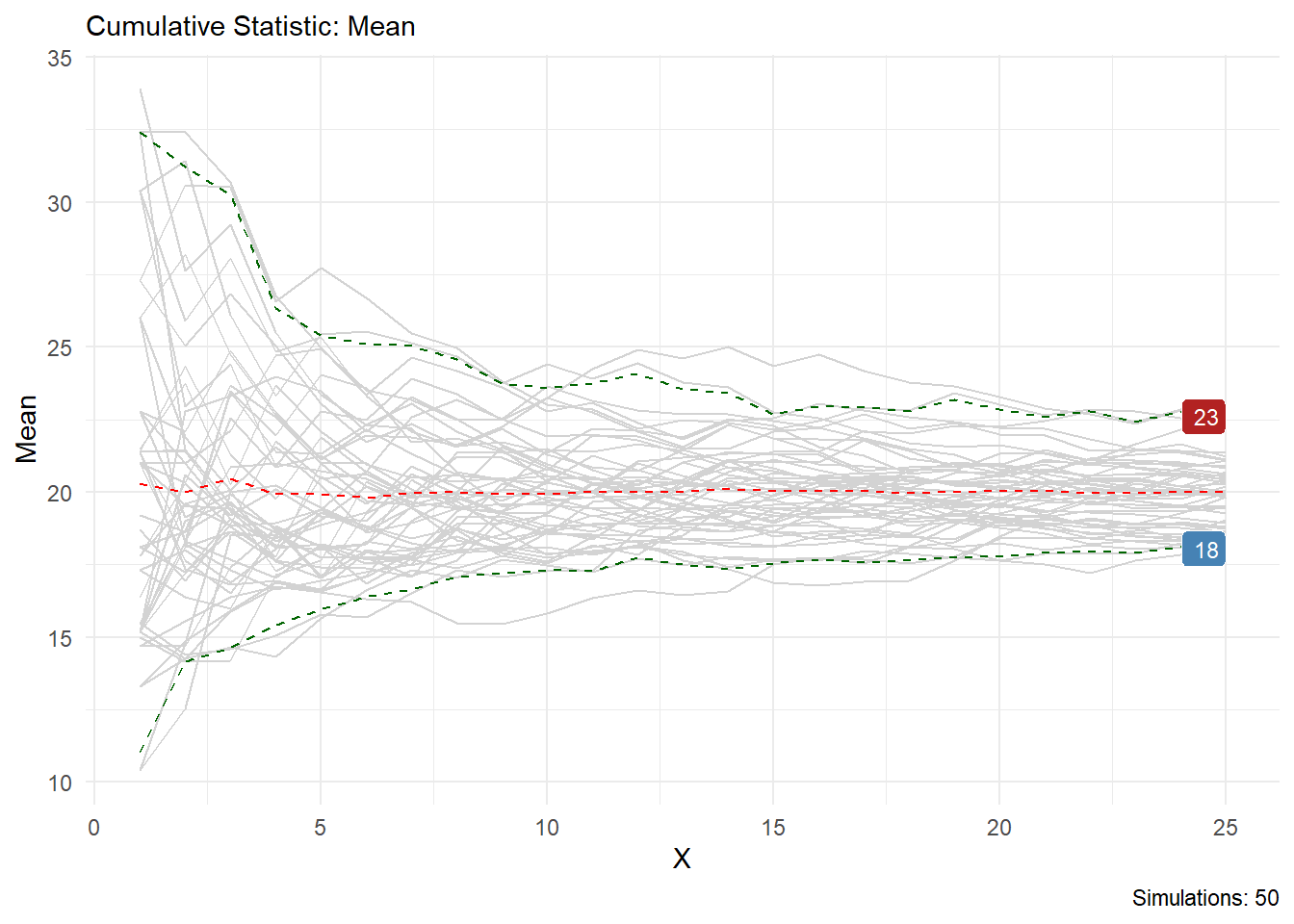

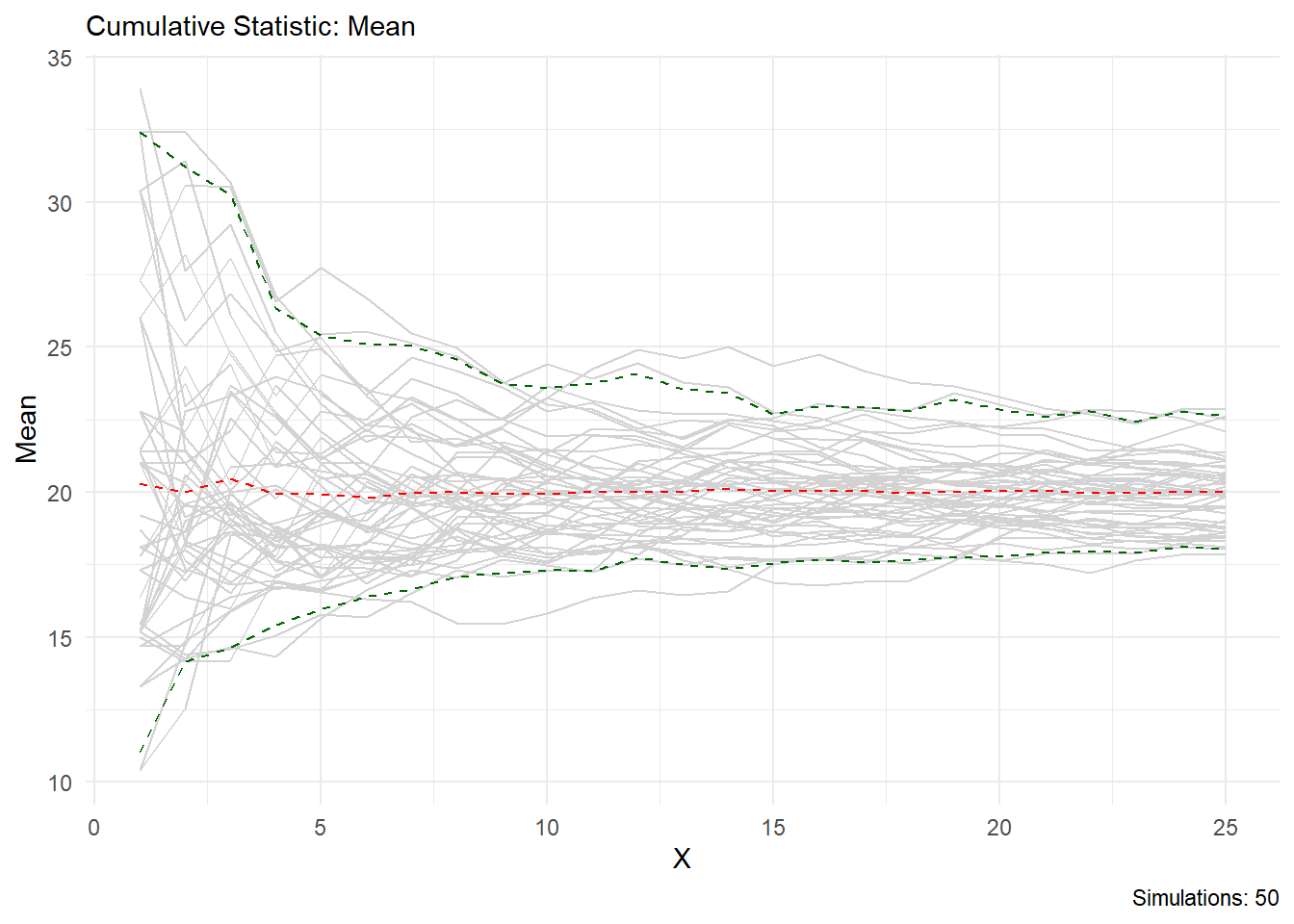
tb %>%
  bootstrap_stat_plot(
    .value = y,
    .show_groups = TRUE,
    .show_ci_labels = FALSE
  )

tb %>%
  bootstrap_stat_plot(.value = y, .interactive = TRUE)

You can see from this output that the statistic you choose is printed in the chart title and on the y axis, the caption will also tell you how many simulations are present. Lets look at skewness as another example.

Cumulative Skewness

sc <- "cskewness"

tb %>%
  bootstrap_stat_plot(.value = y, .stat = sc)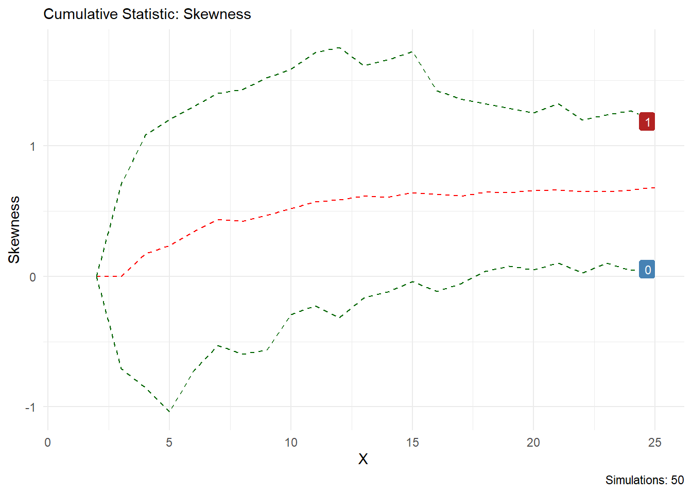

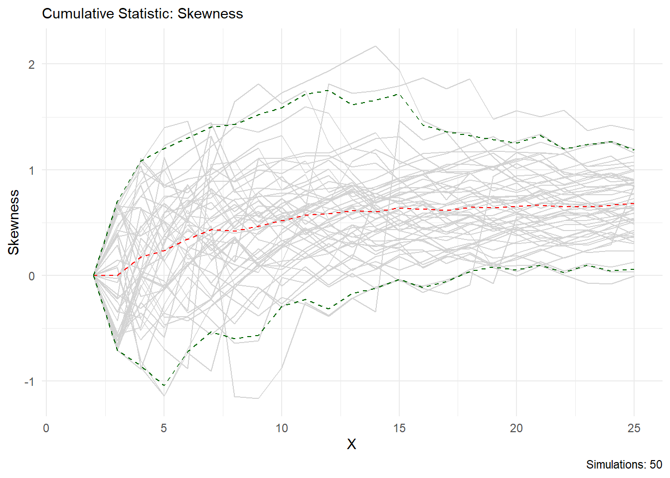
tb %>%
  bootstrap_stat_plot(.value = y, .show_groups = TRUE,
                      .stat = sc)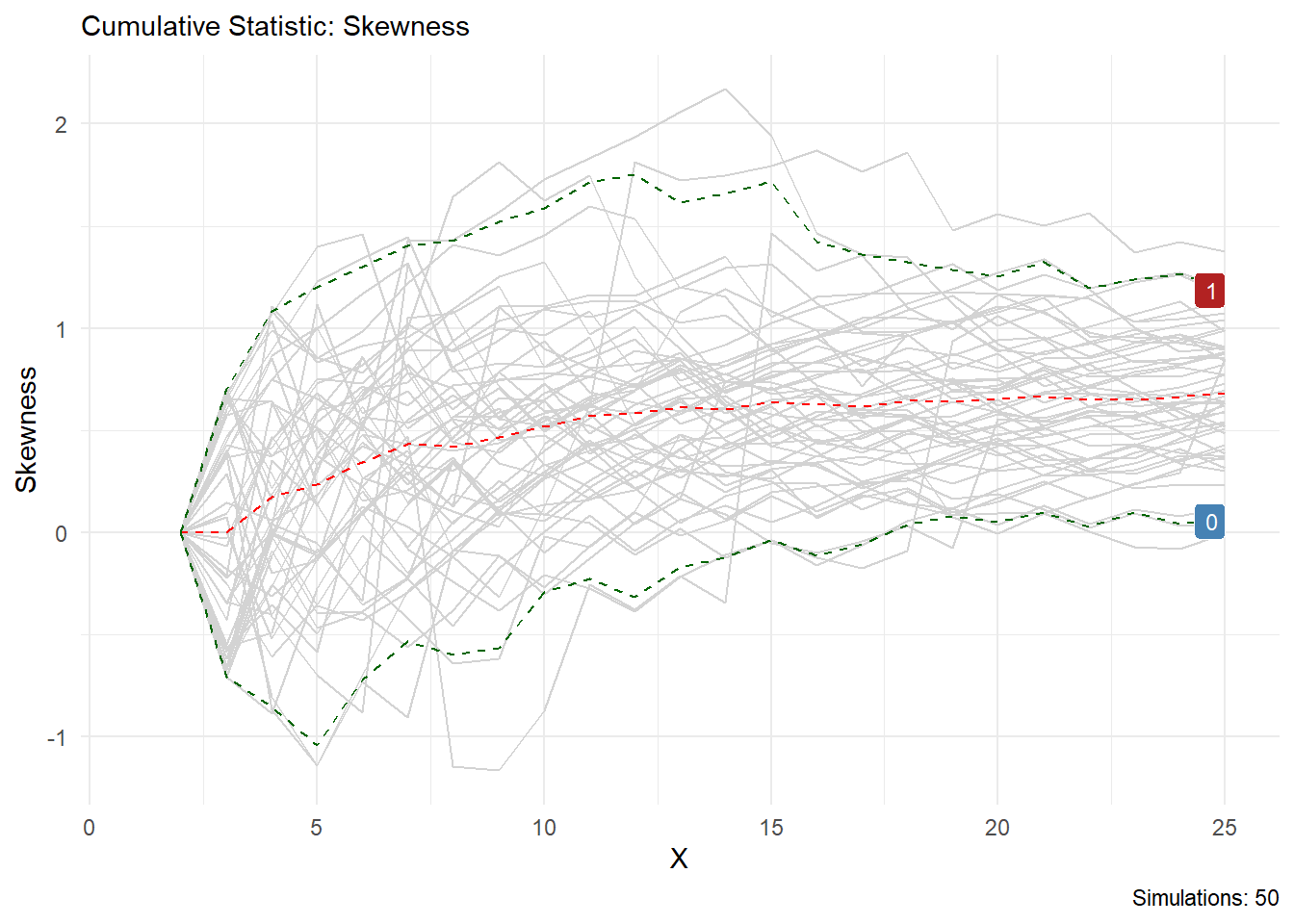

tb %>%
  bootstrap_stat_plot(
    .value = y,
    .stat = sc,
    .show_groups = TRUE,
    .show_ci_labels = FALSE
  )

tb %>%
  bootstrap_stat_plot(.value = y, .interactive = TRUE,
                      .show_groups = TRUE,
                      .stat = sc)

Volia!