package-downloads

CRAN Downloads

Steven P. Sanderson II, MPH - Date: 26 July, 2024

This repo contains the analysis of downloads of my R packages:

• healthyR
• healthyR.data
• healthyR.ts
• healthyR.ai
• healthyverse
• TidyDensity
• tidyAML

All of which follow the “analyses as package” philosophy this repo itself is an R package that can installed using remotes::install_github().

I have forked this project itself from ggcharts-analysis.

While I analyze healthyverse packages here, the functions are written in a way that you can analyze any CRAN package with a slight modification to the download_log function.

This file was last updated on July 26, 2024.

library(packagedownloads)
library(tidyverse)
library(patchwork)
library(timetk)
library(knitr)
library(leaflet)
library(htmltools)
library(tmaptools)
library(mapview)
library(countrycode)
library(htmlwidgets)
library(webshot)
library(rmarkdown)
library(dtplyr)

start_date      <- Sys.Date() - 9 #as.Date("2020-11-15")
end_date        <- Sys.Date() - 2
total_downloads <- download_logs(start_date, end_date)
interactive     <- FALSE
pkg_release_date_tbl()

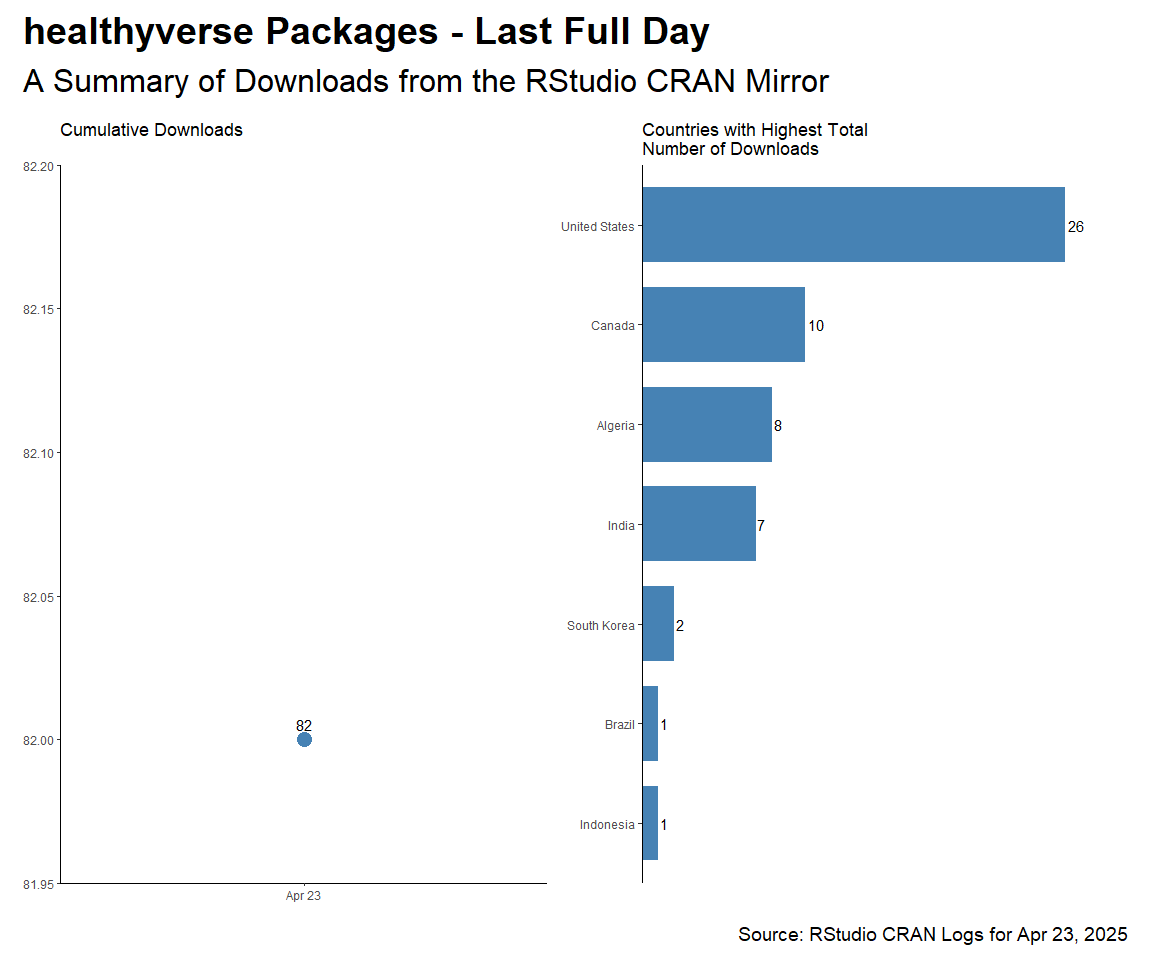
Last Full Day Data

downloads            <- total_downloads |> filter(date == max(date))
daily_downloads      <- compute_daily_downloads(downloads)
downloads_by_country <- compute_downloads_by_country(downloads)

p1 <- plot_cumulative_downloads(daily_downloads)
p2 <- plot_downloads_by_country(downloads_by_country)

f <- function(date) format(date, "%b %d, %Y")
patchwork_theme <- theme_classic(base_size = 24) +
  theme(
    plot.title   = element_text(face = "bold"),
    plot.caption = element_text(size = 14)
  )
p1 + p2 +
  plot_annotation(
    title    = "healthyverse Packages - Last Full Day",
    subtitle = "A Summary of Downloads from the RStudio CRAN Mirror",
    caption  = glue::glue("Source: RStudio CRAN Logs for {f(end_date)}"),
    theme    = patchwork_theme
  )

downloads |>
  count(package, version) |> 
  tidyr::pivot_wider(
    id_cols       = version
    , names_from  = package
    , values_from = n
    , values_fill = 0
    ) |>
  arrange(version) |>
  kable()

version	TidyDensity	healthyR	healthyR.ai	healthyR.data	healthyR.ts	healthyverse	tidyAML
0.0.1	2	0	2	0	0	0	1
0.0.10	0	0	2	0	0	0	0
0.0.11	0	0	2	0	0	0	0
0.0.12	0	0	2	0	0	0	0
0.0.13	0	0	10	0	0	0	0
0.0.2	0	0	2	0	0	0	4
0.0.3	0	0	2	0	0	0	1
0.0.4	0	0	2	0	0	0	1
0.0.5	0	0	2	0	0	0	21
0.0.6	0	0	4	0	0	0	0
0.0.7	0	0	2	0	0	0	0
0.0.8	0	0	2	0	0	0	0
0.0.9	0	0	2	0	0	0	0
0.1.0	0	2	0	0	3	0	0
0.1.1	0	2	0	0	2	0	0
0.1.2	0	2	0	0	2	0	0
0.1.3	0	2	0	0	2	0	0
0.1.4	0	2	0	0	2	0	0
0.1.5	0	2	0	0	2	0	0
0.1.6	0	2	0	0	2	0	0
0.1.7	0	2	0	0	2	0	0
0.1.8	0	5	0	0	2	0	0
0.1.9	0	2	0	0	2	0	0
0.2.0	0	2	0	0	2	0	0
0.2.1	0	2	0	0	2	0	0
0.2.10	0	0	0	0	2	0	0
0.2.11	0	0	0	0	2	0	0
0.2.2	0	15	0	0	2	0	0
0.2.3	0	0	0	0	2	0	0
0.2.4	0	0	0	0	2	0	0
0.2.5	0	0	0	0	2	0	0
0.2.6	0	0	0	0	2	0	0
0.2.7	0	0	0	0	2	0	0
0.2.8	0	0	0	0	6	0	0
0.2.9	0	0	0	0	2	0	0
0.3.0	0	0	0	0	17	0	0
1.0.0	2	0	0	2	0	2	0
1.0.1	8	0	0	2	0	2	0
1.0.2	0	0	0	2	0	2	0
1.0.3	0	0	0	2	0	2	0
1.0.4	0	0	0	0	0	18	0
1.1.0	2	0	0	2	0	0	0
1.1.1	0	0	0	9	0	0	0
1.2.0	2	0	0	0	0	0	0
1.2.1	2	0	0	0	0	0	0
1.2.2	2	0	0	0	0	0	0
1.2.3	2	0	0	0	0	0	0
1.2.4	2	0	0	0	0	0	0
1.2.5	2	0	0	0	0	0	0
1.2.6	2	0	0	0	0	0	0
1.3.0	2	0	0	0	0	0	0
1.4.0	2	0	0	0	0	0	0
1.5.0	24	0	0	0	0	0	0

downloads |>
  count(package, sort = TRUE) |>
  tidyr::pivot_wider(
    names_from = package,
    values_from = n,
    values_fill = 0
  ) |>
  kable()

healthyR.ts	TidyDensity	healthyR	healthyR.ai	tidyAML	healthyverse	healthyR.data
66	56	42	36	28	26	19

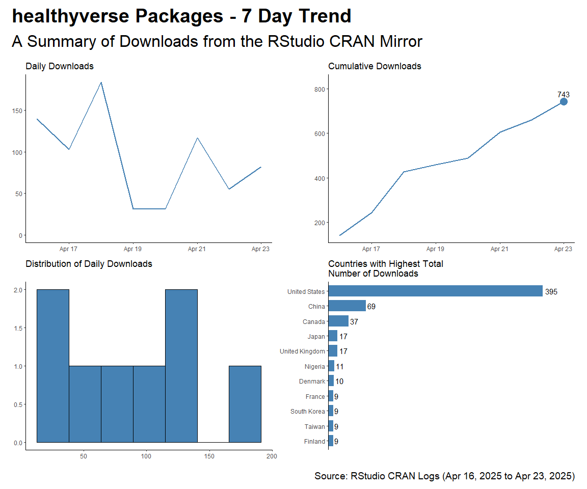
Current Trend

Here are the current 7 day trends for the healthyverse suite of packages.

downloads            <- total_downloads[date >= start_date]
daily_downloads      <- compute_daily_downloads(downloads)
downloads_by_country <- compute_downloads_by_country(downloads)

p1 <- plot_daily_downloads(daily_downloads)
p2 <- plot_cumulative_downloads(daily_downloads)
p3 <- hist_daily_downloads(daily_downloads)
p4 <- plot_downloads_by_country(downloads_by_country)

f <- function(date) format(date, "%b %d, %Y")
patchwork_theme <- theme_classic(base_size = 24) +
  theme(
    plot.title   = element_text(face = "bold"),
    plot.caption = element_text(size = 14)
  )
p1 + p2 + p3 + p4 +
  plot_annotation(
    title    = "healthyverse Packages - 7 Day Trend",
    subtitle = "A Summary of Downloads from the RStudio CRAN Mirror",
    caption  = glue::glue("Source: RStudio CRAN Logs ({f(start_date)} to {f(end_date)})"),
    theme    = patchwork_theme
  )

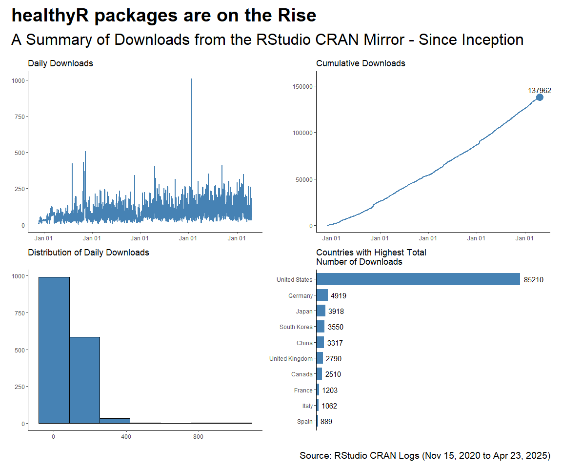
Since Inception

start_date <- as.Date("2020-11-15")

daily_downloads <- compute_daily_downloads(downloads = total_downloads)
downloads_by_country <- compute_downloads_by_country(downloads = total_downloads)

p1 <- plot_daily_downloads(daily_downloads)
p2 <- plot_cumulative_downloads(daily_downloads)
p3 <- hist_daily_downloads(daily_downloads)
p4 <- plot_downloads_by_country(downloads_by_country)

f <- function(date) format(date, "%b %d, %Y")
patchwork_theme <- theme_classic(base_size = 24) +
  theme(
    plot.title   = element_text(face = "bold"),
    plot.caption = element_text(size = 14)
  )
p1 + p2 + p3 + p4 +
  plot_annotation(
    title    = "healthyR packages are on the Rise",
    subtitle = "A Summary of Downloads from the RStudio CRAN Mirror - Since Inception",
    caption  = glue::glue("Source: RStudio CRAN Logs ({f(start_date)} to {f(end_date)})"),
    theme    = patchwork_theme
  )

By Release Date

pkg_tbl <- readRDS("pkg_release_tbl.rds")
dl_tbl <- total_downloads %>%
    filter(
    date != "2024-05-29" &
      !(date == "2024-06-12" & package == "TidyDensity")
    ) |> # bad data on this for some reason
  group_by(package) %>%
  summarise_by_time(
    .date_var = date,
    .by = "week",
    N = n()
  ) %>%
  ungroup() %>%
  select(date, package, N)

dl_tbl %>%
ggplot(aes(date, log1p(N))) +
  theme_bw() +
  geom_point(aes(group = package, color = package), size = 1) +
  geom_line(aes(group = package, color = package)) +
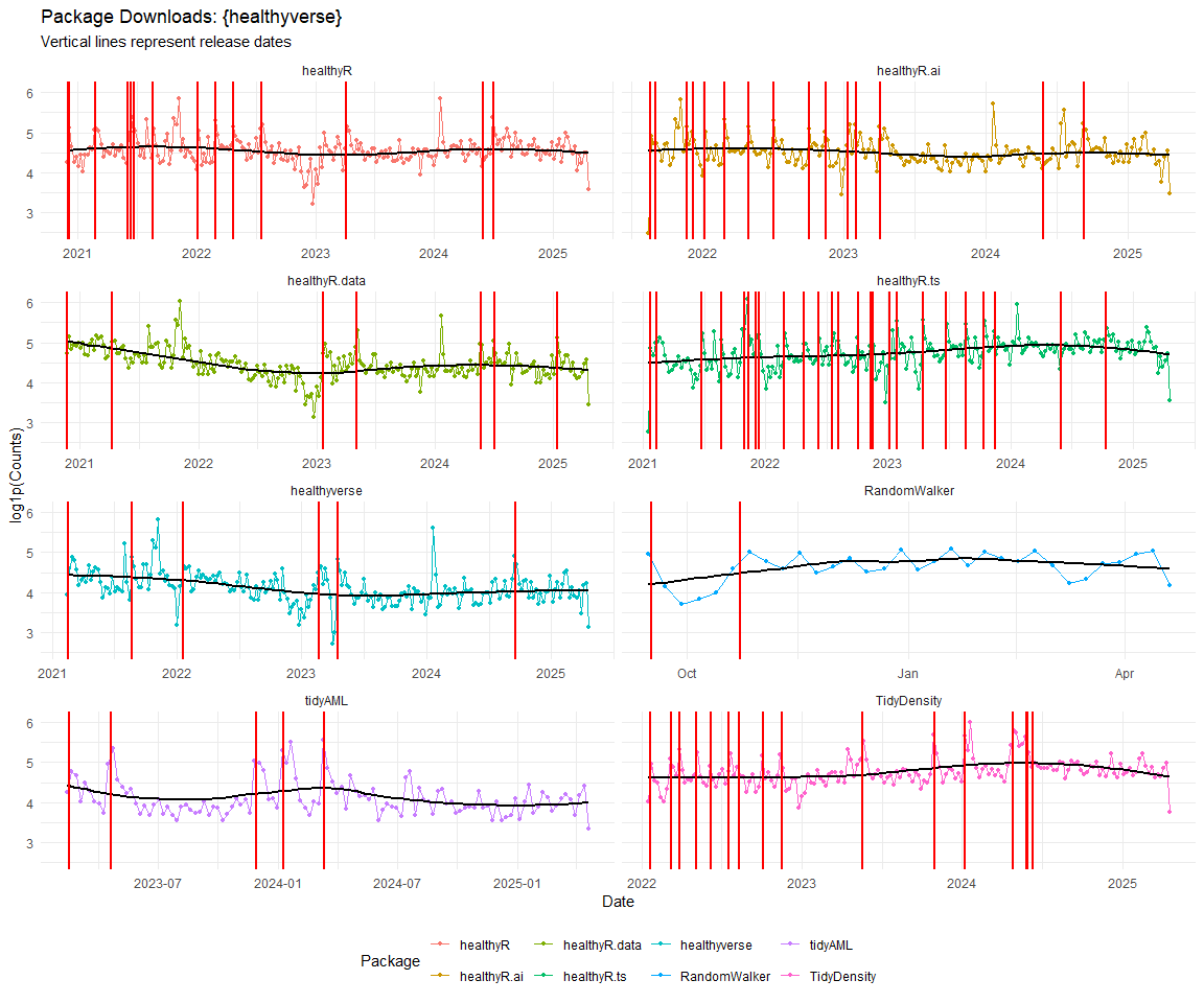
  ggtitle(paste("Package Downloads: {healthyverse}")) +
  geom_smooth(method = "loess", color = "black",  se = FALSE) +
  geom_vline(
    data = pkg_tbl
    , aes(xintercept = as.numeric(date))
    , color = "red"
    , lwd = 1
    , lty = "solid"
  ) +
  facet_wrap(package ~., ncol = 2, scales = "free_x") +
  theme_minimal() +
  labs(
    subtitle = "Vertical lines represent release dates",
    x = "Date",
    y = "log1p(Counts)",
    color = "Package"
  ) +
  theme(legend.position = "bottom")

dl_tbl %>%
  select(date, N) %>%
  summarise_by_time(
    .date_var = date,
    .by = "week",
    Actual = sum(N, na.rm = TRUE)
  ) %>%
  tk_augment_differences(.value = Actual, .differences = 1) %>%
  tk_augment_differences(.value = Actual, .differences = 2) %>%
  rename(velocity = contains("_diff1")) %>%
  rename(acceleration = contains("_diff2")) %>%
  pivot_longer(-date) %>%
  mutate(name = str_to_title(name)) %>%
  mutate(name = as_factor(name)) %>%
  ggplot(aes(x = date, y = log1p(value), group = name)) +
  geom_point(alpha = .2) +
  geom_vline(
    data = pkg_tbl
    , aes(xintercept = as.numeric(date), color = package)
    , lwd = 1
    , lty = "solid"
  ) +
  facet_wrap(name ~ ., ncol = 1, scale = "free") +
  theme_minimal() +
  labs(
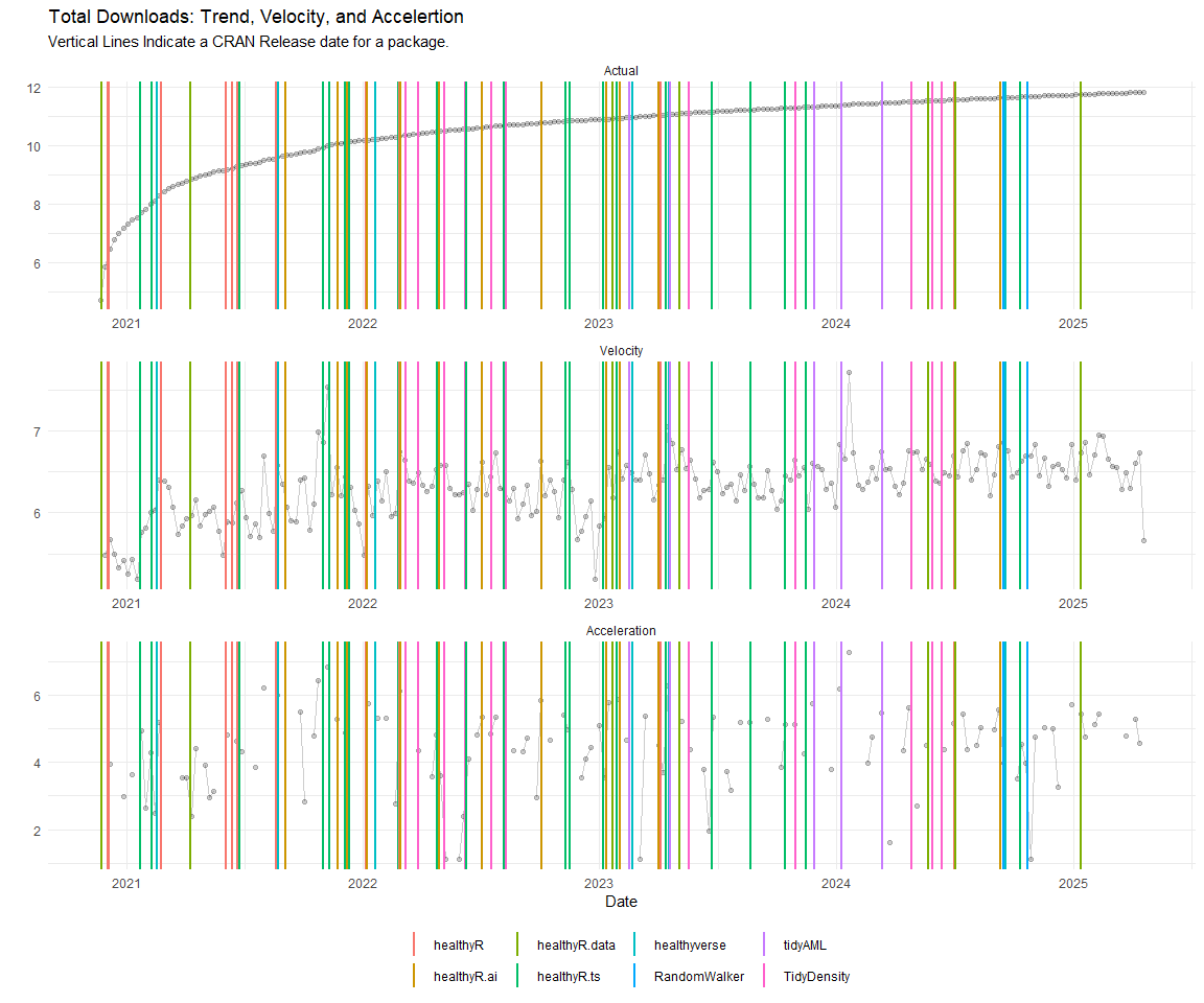
    title = "Total Downloads: Trend, Velocity, and Accelertion",
    subtitle = "Vertical Lines Indicate a CRAN Release date for a package.",
    x = "Date",
    y = "",
    color = ""
  ) +
  theme(legend.position = "bottom")

Map of Downloads

A leaflet map of countries where a package has been downloaded.

mapping_dataset() %>%
  head() %>%
  knitr::kable()

country	latitude	longitude	display_name	icon
United States	39.78373	-100.445882	United States	https://nominatim.openstreetmap.org/ui/mapicons/poi_boundary_administrative.p.20.png
United Kingdom	54.70235	-3.276575	United Kingdom	https://nominatim.openstreetmap.org/ui/mapicons/poi_boundary_administrative.p.20.png
Germany	51.16382	10.447831	Deutschland	https://nominatim.openstreetmap.org/ui/mapicons/poi_boundary_administrative.p.20.png
Hong Kong SAR China	22.35063	114.184916	香港 Hong Kong, 中国	https://nominatim.openstreetmap.org/ui/mapicons/poi_boundary_administrative.p.20.png
Japan	36.57484	139.239418	日本	https://nominatim.openstreetmap.org/ui/mapicons/poi_boundary_administrative.p.20.png
Chile	-31.76134	-71.318770	Chile	https://nominatim.openstreetmap.org/ui/mapicons/poi_boundary_administrative.p.20.png

l <- map_leaflet()
saveWidget(l, "downloads_map.html")
webshot("downloads_map.html", file = "map.png",
        cliprect = "viewport")

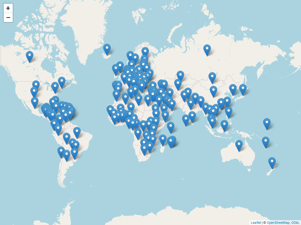
To date there has been downloads in a total of 153 different countries.

Analysis by Package

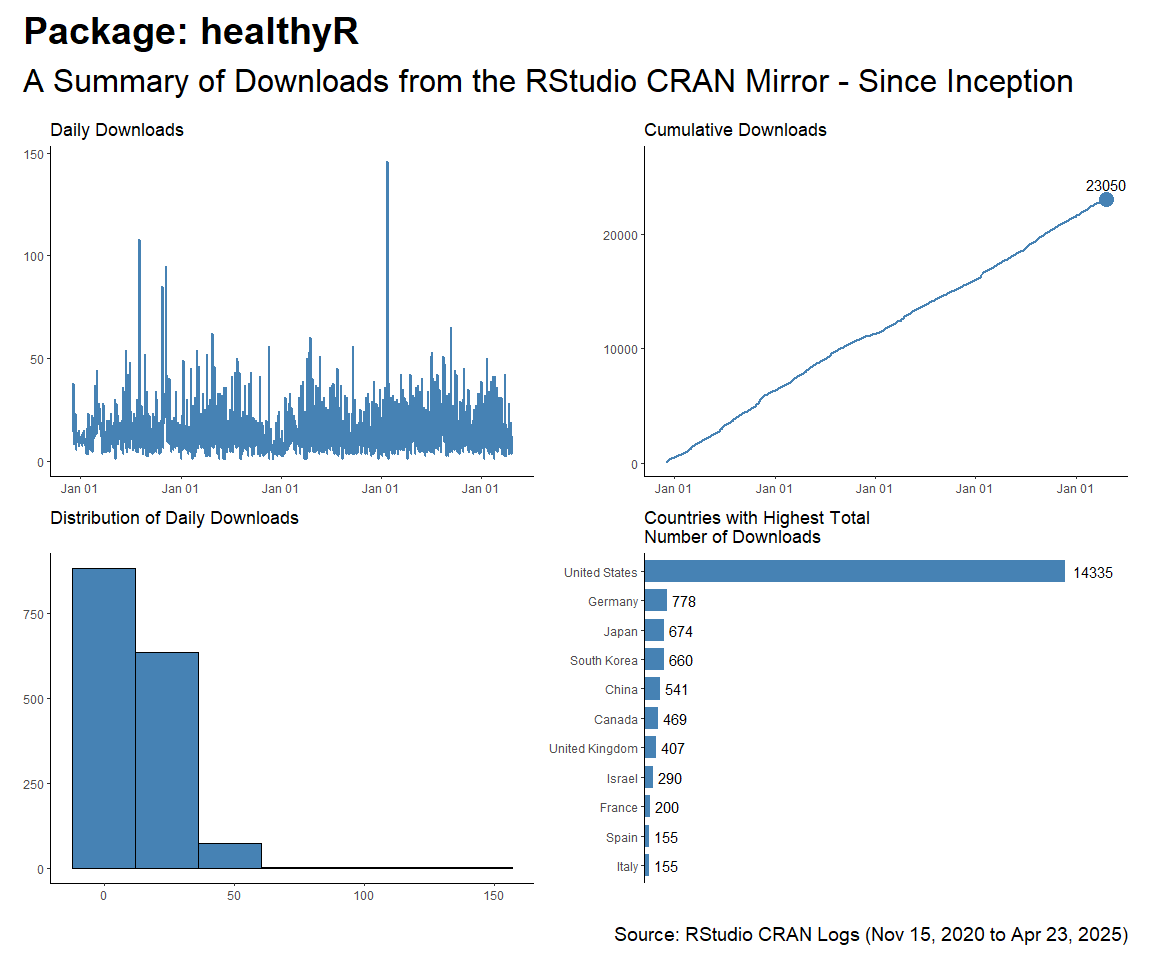
healthyR

start_date <- as.Date("2020-11-15")
pkg <- "healthyR"

daily_downloads <- compute_daily_downloads(
  downloads = total_downloads
  , pkg = pkg)
downloads_by_country <- compute_downloads_by_country(
  downloads = total_downloads
  , pkg = pkg)

p1 <- plot_daily_downloads(daily_downloads)
p2 <- plot_cumulative_downloads(daily_downloads)
p3 <- hist_daily_downloads(daily_downloads)
p4 <- plot_downloads_by_country(downloads_by_country)

f <- function(date) format(date, "%b %d, %Y")
patchwork_theme <- theme_classic(base_size = 24) +
  theme(
    plot.title   = element_text(face = "bold"),
    plot.caption = element_text(size = 14)
  )
p1 + p2 + p3 + p4 +
  plot_annotation(
    title    = glue::glue("Package: {pkg}"),
    subtitle = "A Summary of Downloads from the RStudio CRAN Mirror - Since Inception",
    caption  = glue::glue("Source: RStudio CRAN Logs ({f(start_date)} to {f(end_date)})"),
    theme    = patchwork_theme
  )

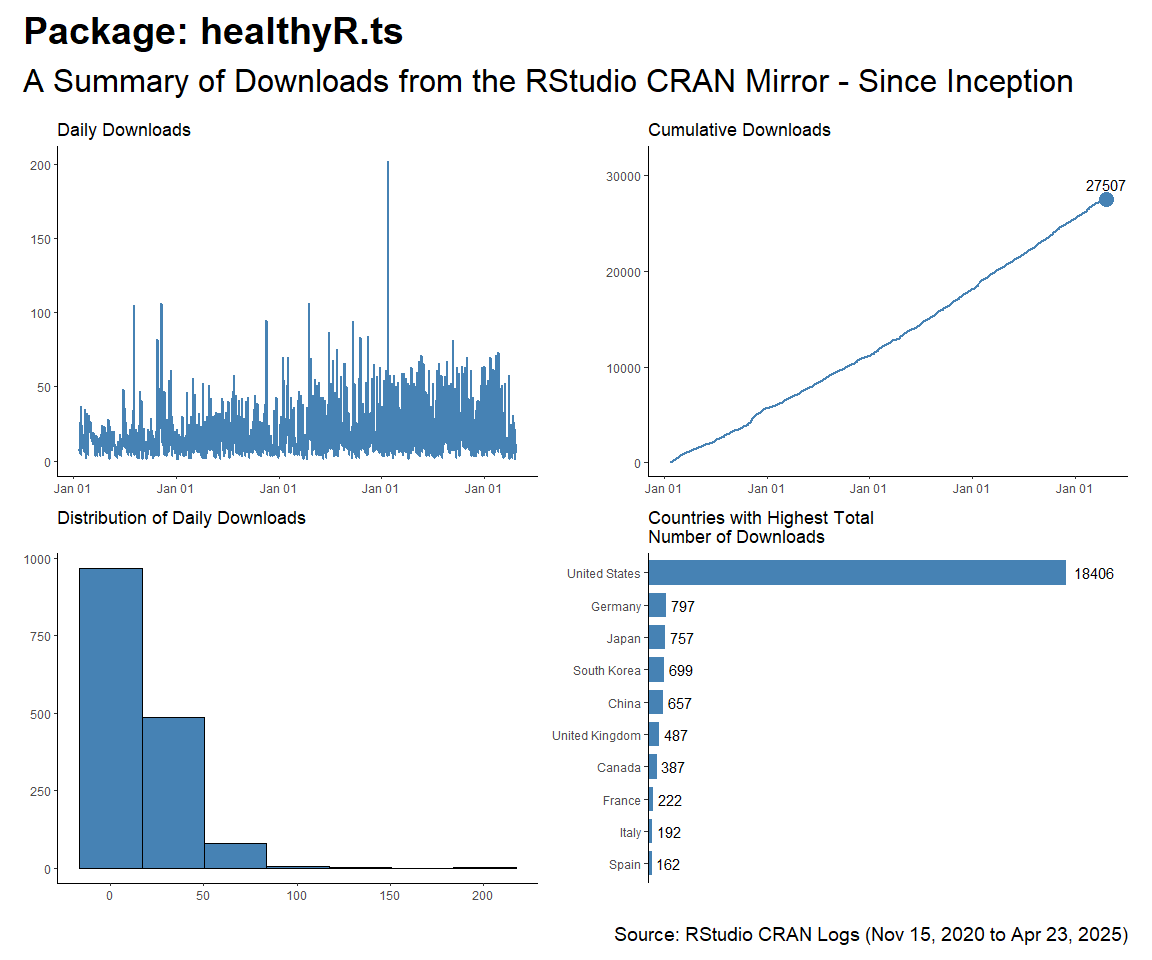
healthyR.ts

start_date <- as.Date("2020-11-15")
pkg <- "healthyR.ts"

daily_downloads <- compute_daily_downloads(
  downloads = total_downloads
  , pkg = pkg)
downloads_by_country <- compute_downloads_by_country(
  downloads = total_downloads
  , pkg = pkg)

p1 <- plot_daily_downloads(daily_downloads)
p2 <- plot_cumulative_downloads(daily_downloads)
p3 <- hist_daily_downloads(daily_downloads)
p4 <- plot_downloads_by_country(downloads_by_country)

f <- function(date) format(date, "%b %d, %Y")
patchwork_theme <- theme_classic(base_size = 24) +
  theme(
    plot.title   = element_text(face = "bold"),
    plot.caption = element_text(size = 14)
  )
p1 + p2 + p3 + p4 +
  plot_annotation(
    title    = glue::glue("Package: {pkg}"),
    subtitle = "A Summary of Downloads from the RStudio CRAN Mirror - Since Inception",
    caption  = glue::glue("Source: RStudio CRAN Logs ({f(start_date)} to {f(end_date)})"),
    theme    = patchwork_theme
  )

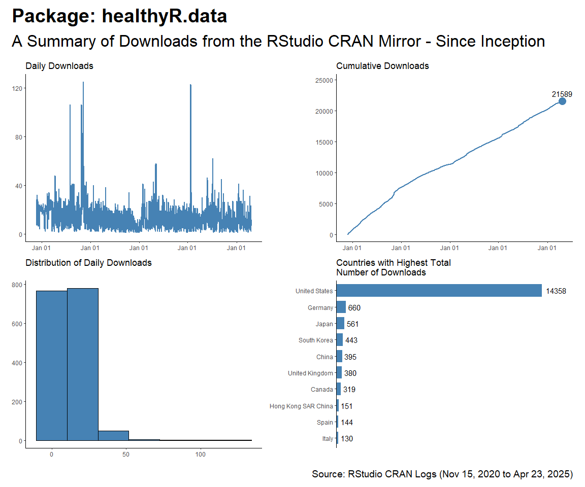
healthyR.data

start_date <- as.Date("2020-11-15")
pkg <- "healthyR.data"

daily_downloads <- compute_daily_downloads(
  downloads = total_downloads
  , pkg = pkg)
downloads_by_country <- compute_downloads_by_country(
  downloads = total_downloads
  , pkg = pkg)

p1 <- plot_daily_downloads(daily_downloads)
p2 <- plot_cumulative_downloads(daily_downloads)
p3 <- hist_daily_downloads(daily_downloads)
p4 <- plot_downloads_by_country(downloads_by_country)

f <- function(date) format(date, "%b %d, %Y")
patchwork_theme <- theme_classic(base_size = 24) +
  theme(
    plot.title   = element_text(face = "bold"),
    plot.caption = element_text(size = 14)
  )
p1 + p2 + p3 + p4 +
  plot_annotation(
    title    = glue::glue("Package: {pkg}"),
    subtitle = "A Summary of Downloads from the RStudio CRAN Mirror - Since Inception",
    caption  = glue::glue("Source: RStudio CRAN Logs ({f(start_date)} to {f(end_date)})"),
    theme    = patchwork_theme
  )

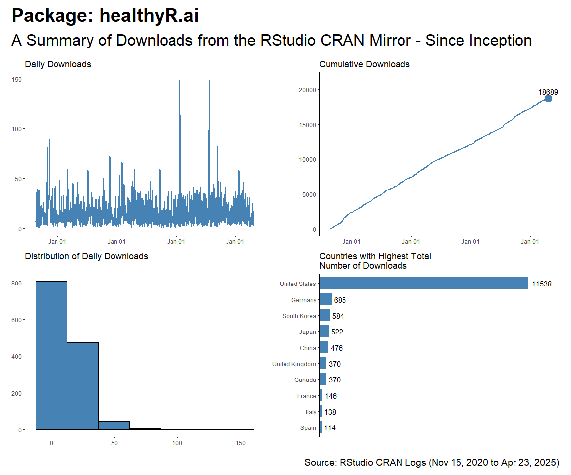
healthyR.ai

start_date <- as.Date("2020-11-15")
pkg <- "healthyR.ai"

daily_downloads <- compute_daily_downloads(
  downloads = total_downloads
  , pkg = pkg)
downloads_by_country <- compute_downloads_by_country(
  downloads = total_downloads
  , pkg = pkg)

p1 <- plot_daily_downloads(daily_downloads)
p2 <- plot_cumulative_downloads(daily_downloads)
p3 <- hist_daily_downloads(daily_downloads)
p4 <- plot_downloads_by_country(downloads_by_country)

f <- function(date) format(date, "%b %d, %Y")
patchwork_theme <- theme_classic(base_size = 24) +
  theme(
    plot.title   = element_text(face = "bold"),
    plot.caption = element_text(size = 14)
  )
p1 + p2 + p3 + p4 +
  plot_annotation(
    title    = glue::glue("Package: {pkg}"),
    subtitle = "A Summary of Downloads from the RStudio CRAN Mirror - Since Inception",
    caption  = glue::glue("Source: RStudio CRAN Logs ({f(start_date)} to {f(end_date)})"),
    theme    = patchwork_theme
  )

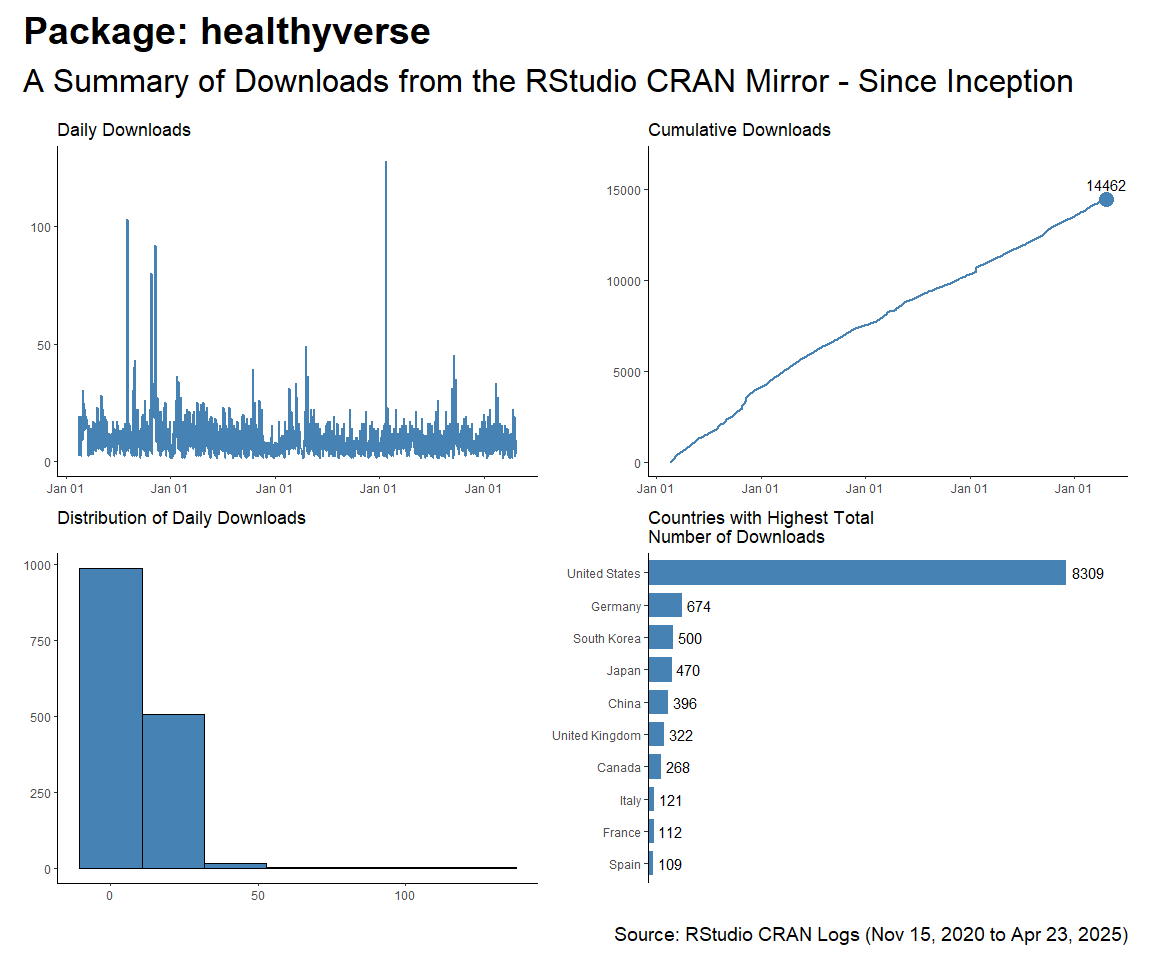
healthyverse

start_date <- as.Date("2020-11-15")
pkg <- "healthyverse"

daily_downloads <- compute_daily_downloads(
  downloads = total_downloads
  , pkg = pkg)
downloads_by_country <- compute_downloads_by_country(
  downloads = total_downloads
  , pkg = pkg)

p1 <- plot_daily_downloads(daily_downloads)
p2 <- plot_cumulative_downloads(daily_downloads)
p3 <- hist_daily_downloads(daily_downloads)
p4 <- plot_downloads_by_country(downloads_by_country)

f <- function(date) format(date, "%b %d, %Y")
patchwork_theme <- theme_classic(base_size = 24) +
  theme(
    plot.title   = element_text(face = "bold"),
    plot.caption = element_text(size = 14)
  )
p1 + p2 + p3 + p4 +
  plot_annotation(
    title    = glue::glue("Package: {pkg}"),
    subtitle = "A Summary of Downloads from the RStudio CRAN Mirror - Since Inception",
    caption  = glue::glue("Source: RStudio CRAN Logs ({f(start_date)} to {f(end_date)})"),
    theme    = patchwork_theme
  )

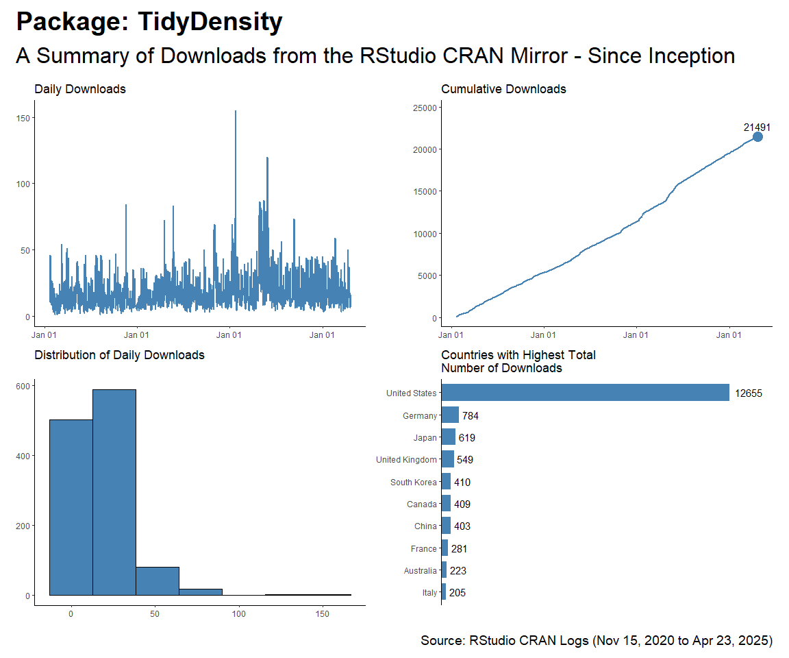
TidyDensity

start_date <- as.Date("2020-11-15")
pkg <- "TidyDensity"

daily_downloads <- compute_daily_downloads(
  downloads = total_downloads
  , pkg = pkg)
downloads_by_country <- compute_downloads_by_country(
  downloads = total_downloads
  , pkg = pkg)

p1 <- plot_daily_downloads(daily_downloads)
p2 <- plot_cumulative_downloads(daily_downloads)
p3 <- hist_daily_downloads(daily_downloads)
p4 <- plot_downloads_by_country(downloads_by_country)

f <- function(date) format(date, "%b %d, %Y")
patchwork_theme <- theme_classic(base_size = 24) +
  theme(
    plot.title   = element_text(face = "bold"),
    plot.caption = element_text(size = 14)
  )
p1 + p2 + p3 + p4 +
  plot_annotation(
    title    = glue::glue("Package: {pkg}"),
    subtitle = "A Summary of Downloads from the RStudio CRAN Mirror - Since Inception",
    caption  = glue::glue("Source: RStudio CRAN Logs ({f(start_date)} to {f(end_date)})"),
    theme    = patchwork_theme
  )

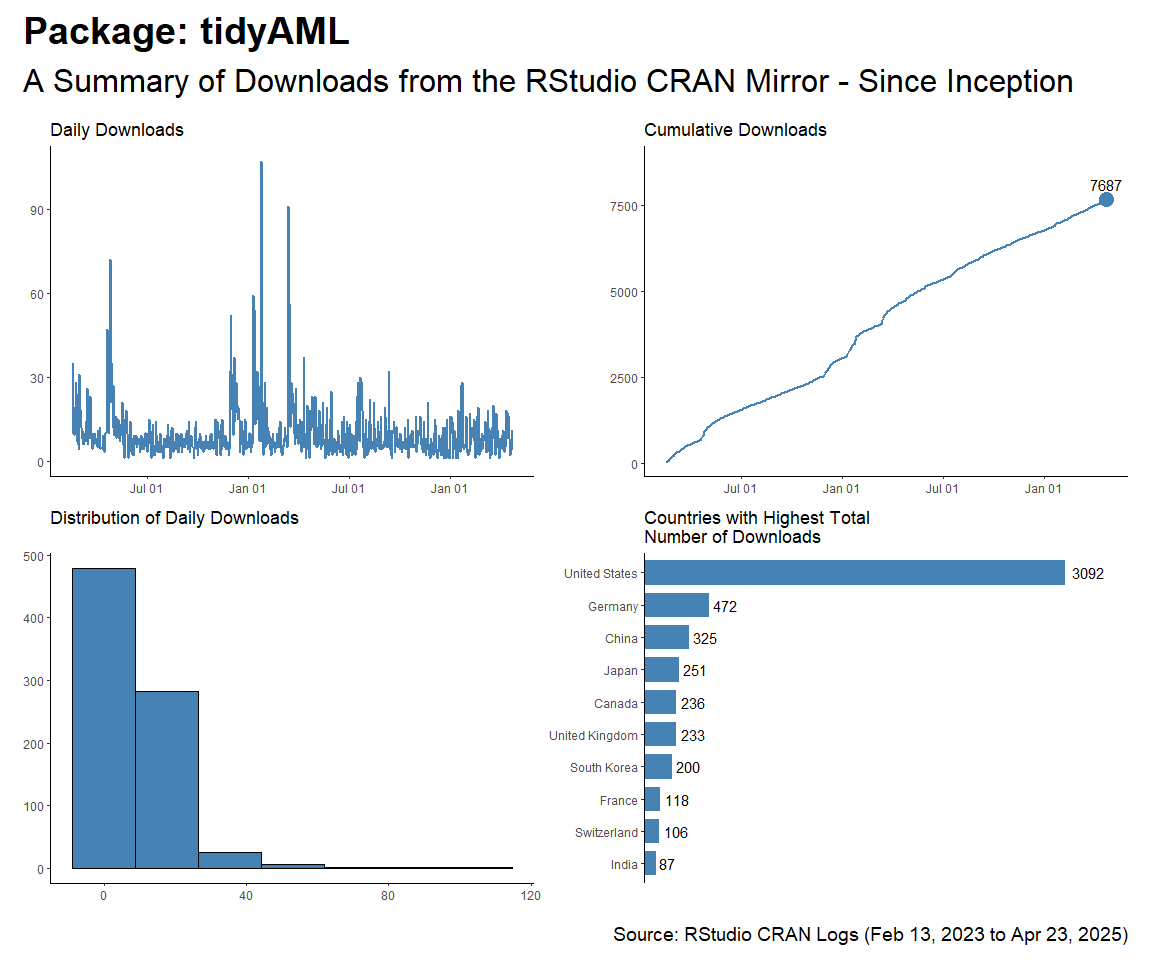
tidyAML

start_date <- as.Date("2023-02-13")
pkg <- "tidyAML"

daily_downloads <- compute_daily_downloads(
  downloads = total_downloads
  , pkg = pkg)
downloads_by_country <- compute_downloads_by_country(
  downloads = total_downloads
  , pkg = pkg)

p1 <- plot_daily_downloads(daily_downloads)
p2 <- plot_cumulative_downloads(daily_downloads)
p3 <- hist_daily_downloads(daily_downloads)
p4 <- plot_downloads_by_country(downloads_by_country)

f <- function(date) format(date, "%b %d, %Y")
patchwork_theme <- theme_classic(base_size = 24) +
  theme(
    plot.title   = element_text(face = "bold"),
    plot.caption = element_text(size = 14)
  )
p1 + p2 + p3 + p4 +
  plot_annotation(
    title    = glue::glue("Package: {pkg}"),
    subtitle = "A Summary of Downloads from the RStudio CRAN Mirror - Since Inception",
    caption  = glue::glue("Source: RStudio CRAN Logs ({f(start_date)} to {f(end_date)})"),
    theme    = patchwork_theme
  )

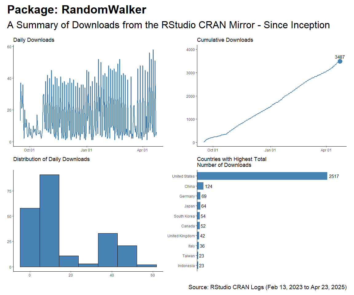
Table Data

Downloads by Package and Version

total_downloads %>% 
  count(package, version) %>% 
  tidyr::pivot_wider(
    id_cols       = version
    , names_from  = package
    , values_from = n
    , values_fill = 0
    ) %>%
  arrange(version) %>%
  kable()

version	TidyDensity	healthyR	healthyR.ai	healthyR.data	healthyR.ts	healthyverse	tidyAML
0.0.1	1216	0	534	0	0	0	854
0.0.10	0	0	663	0	0	0	0
0.0.11	0	0	501	0	0	0	0
0.0.12	0	0	753	0	0	0	0
0.0.13	0	0	3568	0	0	0	0
0.0.13.tar.gz%20H	0	0	5	0	0	0	0
0.0.2	0	0	1786	0	0	0	1918
0.0.3	0	0	546	0	0	0	615
0.0.4	0	0	631	0	0	0	890
0.0.5	0	0	1211	0	0	0	1330
0.0.6	0	0	2094	0	0	0	0
0.0.7	0	0	882	0	0	0	0
0.0.8	0	0	1009	0	0	0	0
0.0.9	0	0	796	0	0	0	0
0.1.0	0	431	0	0	656	0	0
0.1.1	0	1479	0	0	2176	0	0
0.1.2	0	1704	0	0	1170	0	0
0.1.3	0	504	0	0	1287	0	0
0.1.4	0	552	0	0	857	0	0
0.1.5	0	1198	0	0	696	0	0
0.1.6	0	2403	0	0	432	0	0
0.1.7	0	1190	0	0	1427	0	0
0.1.8	0	1840	0	0	1812	0	0
0.1.9	0	1059	0	0	667	0	0
0.2.0	0	2307	0	0	671	0	0
0.2.1	0	4159	0	0	486	0	0
0.2.1.tar.gz%20HT	0	5	0	0	0	0	0
0.2.10	0	0	0	0	569	0	0
0.2.11	0	0	0	0	604	0	0
0.2.2	0	354	0	0	711	0	0
0.2.2.tar.gz%20	0	0	0	0	10	0	0
0.2.3	0	0	0	0	720	0	0
0.2.4	0	0	0	0	342	0	0
0.2.5	0	0	0	0	639	0	0
0.2.6	0	0	0	0	500	0	0
0.2.7	0	0	0	0	889	0	0
0.2.8	0	0	0	0	1766	0	0
0.2.9	0	0	0	0	785	0	0
0.3.0	0	0	0	0	2334	0	0
0.3.0.tar.gz%20H	0	0	0	0	5	0	0
1.0.0	580	0	0	3056	0	2532	0
1.0.1	1650	0	0	9811	0	2337	0
1.0.2	0	0	0	1666	0	3683	0
1.0.3	0	0	0	3082	0	522	0
1.0.4	0	0	0	0	0	3016	0
1.1.0	616	0	0	499	0	0	0
1.1.1	0	0	0	270	0	0	0
1.2.0	702	0	0	0	0	0	0
1.2.1	518	0	0	0	0	0	0
1.2.2	733	0	0	0	0	0	0
1.2.3	765	0	0	0	0	0	0
1.2.4	2779	0	0	0	0	0	0
1.2.5	1957	0	0	0	0	0	0
1.2.6	1155	0	0	0	0	0	0
1.3.0	1723	0	0	0	0	0	0
1.4.0	1168	0	0	0	0	0	0
1.4.0.tar.gz%20H	1	0	0	0	0	0	0
1.5.0	1014	0	0	0	0	0	0
1.5.0.tar.gz%20HT	3	0	0	0	0	0	0

total_downloads %>%
  count(package, sort = TRUE) %>%
  tidyr::pivot_wider(
    names_from = package,
    values_from = n
  ) |>
  kable()

healthyR.ts	healthyR	healthyR.data	TidyDensity	healthyR.ai	healthyverse	tidyAML
22211	19185	18384	16580	14979	12090	5607

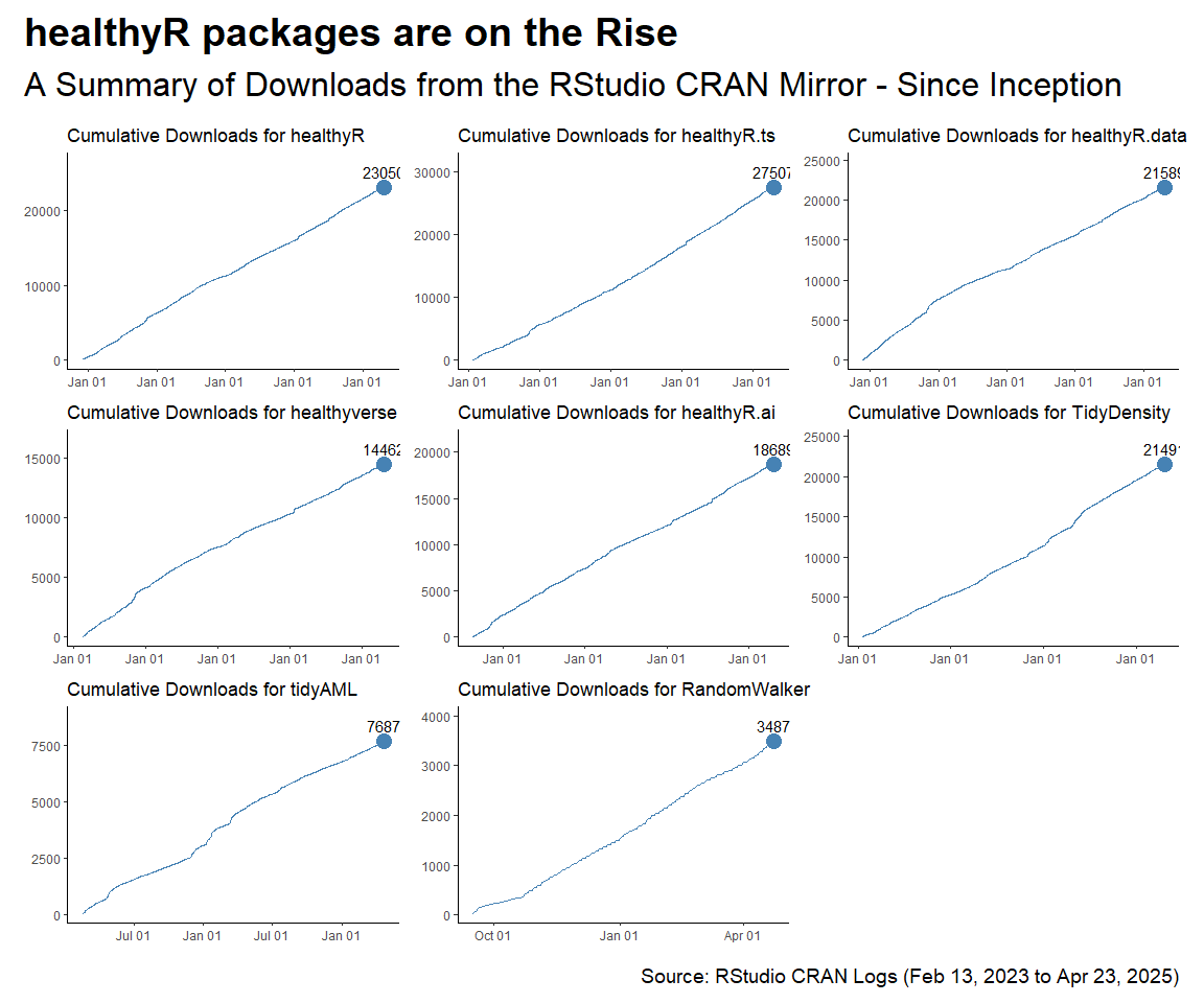
Cumulative Downloads by Package

p1 <- plot_cumulative_downloads_pkg(total_downloads, pkg = "healthyR")
p2 <- plot_cumulative_downloads_pkg(total_downloads, pkg = "healthyR.ts")
p3 <- plot_cumulative_downloads_pkg(total_downloads, pkg = "healthyR.data")
p4 <- plot_cumulative_downloads_pkg(total_downloads, pkg = "healthyverse")
p5 <- plot_cumulative_downloads_pkg(total_downloads, pkg = "healthyR.ai")
p6 <- plot_cumulative_downloads_pkg(total_downloads, pkg = "TidyDensity")
p7 <- plot_cumulative_downloads_pkg(total_downloads, pkg = "tidyAML")

f <- function(date) format(date, "%b %d, %Y")
patchwork_theme <- theme_classic(base_size = 24) +
  theme(
    plot.title   = element_text(face = "bold"),
    plot.caption = element_text(size = 14)
  )
p1 + p2 + p3 + p4 + p5 + p6 + p7 +
  plot_annotation(
    title    = "healthyR packages are on the Rise",
    subtitle = "A Summary of Downloads from the RStudio CRAN Mirror - Since Inception",
    caption  = glue::glue("Source: RStudio CRAN Logs ({f(start_date)} to {f(end_date)})"),
    theme    = patchwork_theme
  )

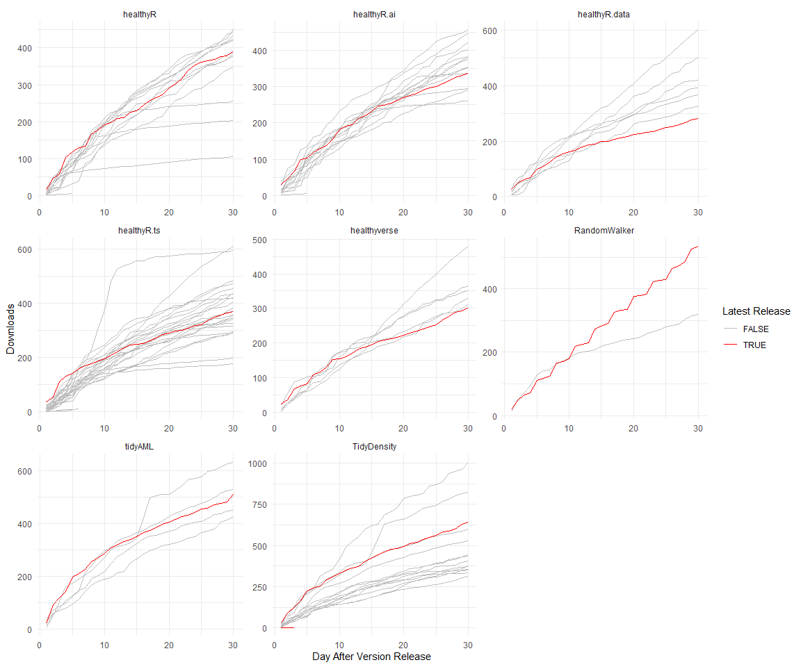
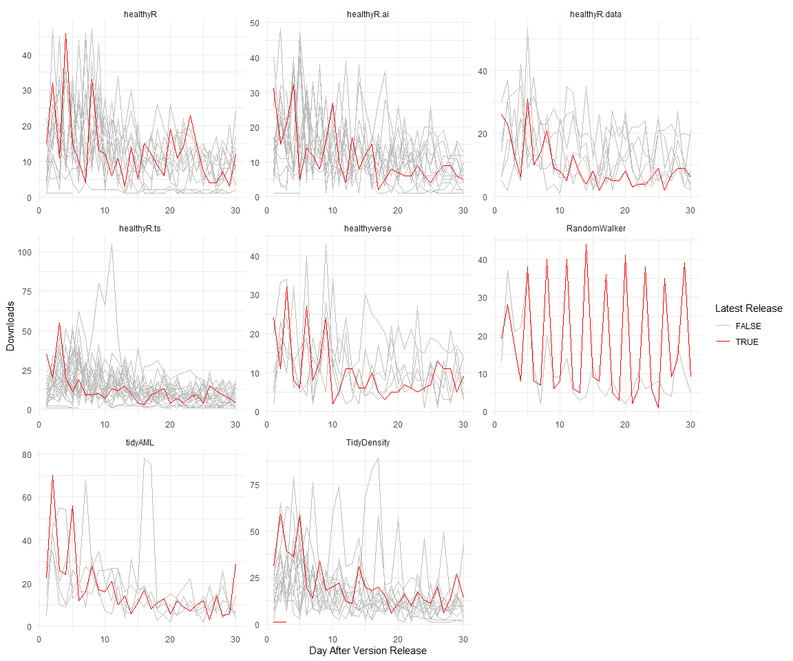
Thirty Day Run Post Release

pkg_rel <- readRDS("pkg_release_tbl.rds") |>
  # Filter out bad data, not sure why it occurrs. 
  filter(
    date != "2024-05-29" &
      !(date == "2024-06-12" & package == "TidyDensity")
    ) |>
  arrange(date) |>
  group_by(package) |>
  mutate(rel_no = row_number()) |>
  ungroup()

thirty_day_runup_tbl <- total_downloads |>
  lazy_dt() |>
  select(date, package, version) |>
  group_by(date, package, version) |>
  summarise(dl_count = n()) |>
  ungroup() |>
  arrange(date) |>
  group_by(package, version) |>
  mutate(rec_no = row_number()) |>
  mutate(cum_dl = cumsum(dl_count)) |>
  filter(rec_no < 31) |>
  ungroup() |>
  mutate(pkg_ver = paste0(package, "-", version)) |>
  collect()

release_tbl <- left_join(
  x = thirty_day_runup_tbl,
  y = pkg_rel
) |>
  group_by(package) |>
  fill(release_record, .direction = "down") |>
  fill(rel_no, .direction = "down") |>
  mutate(
    release_record = as.factor(release_record),
    rel_no = as.factor(rel_no)
  ) |>
  ungroup()

latest_group_tbl <- release_tbl |>
  group_by(package) |> 
  arrange(date, rec_no) |>
  mutate(group_no = as.numeric(rel_no)) |> 
  filter(group_no == max(group_no)) |>
  ungroup()

joined_tbl <- left_join(
  x = thirty_day_runup_tbl, 
  y = latest_group_tbl
  ) |>
  mutate(group_no = ifelse(is.na(group_no), FALSE, TRUE))

joined_tbl |>
  ggplot(aes(x = rec_no, y = dl_count, group = as.factor(pkg_ver))) +
  facet_wrap(~ package, scales = "free", ncol = 3) +
  geom_line(aes(col = group_no)) +
  scale_color_manual(values = c("FALSE" = "grey", "TRUE" = "red")) +
  theme_minimal() +
  labs(
    y = "Downloads",
    x = "Day After Version Release",
    col = "Latest Release"
  )

joined_tbl |>
  ggplot(aes(x = rec_no, y = cum_dl, group = as.factor(pkg_ver))) +
  facet_wrap(~ package, scales = "free", ncol = 3) +
  geom_line(aes(col = group_no)) +
  scale_color_manual(values = c("FALSE" = "grey", "TRUE" = "red")) +
  theme_minimal() +
  labs(
    y = "Downloads",
    x = "Day After Version Release",
    col = "Latest Release"
  )