The goal of healthyR.ts is to provide a consistent verb framework for performing time series analysis and forecasting on both administrative and clinical hospital data.
Installation
You can install the released version of healthyR.ts from CRAN with:
install.packages("healthyR.ts")And the development version from GitHub with:
# install.packages("devtools")
devtools::install_github("spsanderson/healthyR.ts")
Example
This is a basic example which shows you how to generate random walk data.
library(healthyR.ts)
library(ggplot2)

df <- ts_random_walk()

head(df)
#> # A tibble: 6 × 4
#>     run     x        y cum_y
#>   <dbl> <dbl>    <dbl> <dbl>
#> 1     1     1 0.0521   1052.
#> 2     1     2 0.000486 1053.
#> 3     1     3 0.0567   1112.
#> 4     1     4 0.125    1252.
#> 5     1     5 0.0825   1355.
#> 6     1     6 0.00340  1360.
Now that the data has been generated, lets take a look at it.
df %>%
   ggplot(
       mapping = aes(
           x = x
           , y = cum_y
           , color = factor(run)
           , group = factor(run)
        )
    ) +
    geom_line(alpha = 0.8) +
    ts_random_walk_ggplot_layers(df)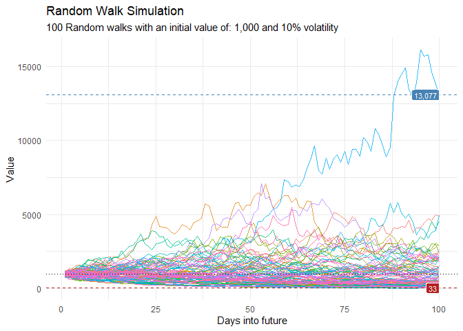
That is still pretty noisy, so lets see this in a different way. Lets clear this up a bit to make it easier to see the full range of the possible volatility of the random walks.
library(dplyr)
library(ggplot2)

df %>%
    group_by(x) %>%
    summarise(
        min_y = min(cum_y),
        max_y = max(cum_y)
    ) %>%
    ggplot(
        aes(x = x)
    ) +
    geom_line(aes(y = max_y), color = "steelblue") +
    geom_line(aes(y = min_y), color = "firebrick") +
    geom_ribbon(aes(ymin = min_y, ymax = max_y), alpha = 0.2) +
    ts_random_walk_ggplot_layers(df)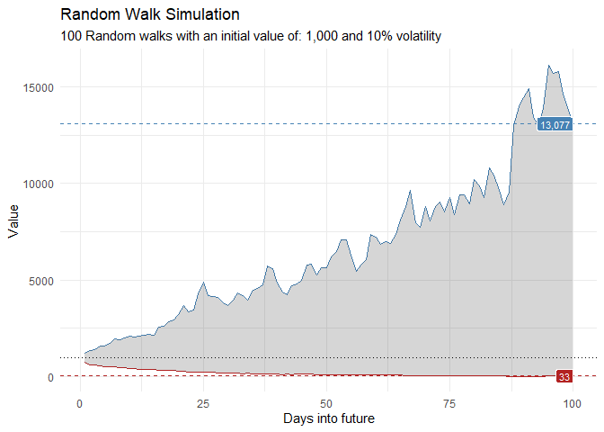
This package comes with a wide variety of functions from Data Generators to Statistics functions. The function ts_random_walk() in the above example is a Data Generator.
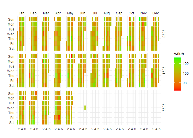
Let’s take a look at a plotting function.
data_tbl <- data.frame(
  date_col = seq.Date(
    from = as.Date("2020-01-01"),
    to   = as.Date("2022-06-01"),
    length.out = 365*2 + 180
    ),
  value = rnorm(365*2+180, mean = 100)
)

ts_calendar_heatmap_plot(
  .data          = data_tbl
  , .date_col    = date_col
  , .value_col   = value
  , .interactive = FALSE
)
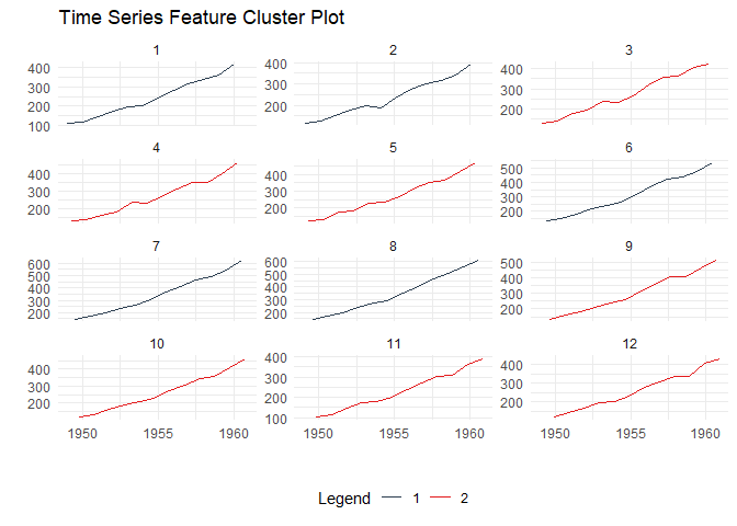
Time Series Clustering via Features:
data_tbl <- ts_to_tbl(AirPassengers) %>%
  mutate(group_id = rep(1:12, 12))

output <- ts_feature_cluster(
  .data = data_tbl,
  .date_col = date_col,
  .value_col = value,
  group_id,
  .features = c("acf_features","entropy"),
  .scale = TRUE,
  .prefix = "ts_",
  .centers = 3
)

ts_feature_cluster_plot(
  .data = output,
  .date_col = date_col,
  .value_col = value,
  .center = 2,
  group_id
)

#>
#> $plot$plotly_plot
#>
#>
#> $data
#> $data$original_data
#> # A tibble: 144 × 4
#>    index     date_col   value group_id
#>    <yearmon> <date>     <dbl>    <int>
#>  1 Jan 1949  1949-01-01   112        1
#>  2 Feb 1949  1949-02-01   118        2
#>  3 Mar 1949  1949-03-01   132        3
#>  4 Apr 1949  1949-04-01   129        4
#>  5 May 1949  1949-05-01   121        5
#>  6 Jun 1949  1949-06-01   135        6
#>  7 Jul 1949  1949-07-01   148        7
#>  8 Aug 1949  1949-08-01   148        8
#>  9 Sep 1949  1949-09-01   136        9
#> 10 Oct 1949  1949-10-01   119       10
#> # ℹ 134 more rows
#>
#> $data$kmm_data_tbl
#> # A tibble: 3 × 3
#>   centers k_means  glance
#>     <int> <list>   <list>
#> 1       1 <kmeans> <tibble [1 × 4]>
#> 2       2 <kmeans> <tibble [1 × 4]>
#> 3       3 <kmeans> <tibble [1 × 4]>
#>
#> $data$user_item_tbl
#> # A tibble: 12 × 8
#>    group_id ts_x_acf1 ts_x_acf10 ts_diff1_acf1 ts_diff1_acf10 ts_diff2_acf1
#>       <int>     <dbl>      <dbl>         <dbl>          <dbl>         <dbl>
#>  1        1     0.741       1.55       -0.0995          0.474       -0.182
#>  2        2     0.730       1.50       -0.0155          0.654       -0.147
#>  3        3     0.766       1.62       -0.471           0.562       -0.620
#>  4        4     0.715       1.46       -0.253           0.457       -0.555
#>  5        5     0.730       1.48       -0.372           0.417       -0.649
#>  6        6     0.751       1.61        0.122           0.646        0.0506
#>  7        7     0.745       1.58        0.260           0.236       -0.303
#>  8        8     0.761       1.60        0.319           0.419       -0.319
#>  9        9     0.747       1.59       -0.235           0.191       -0.650
#> 10       10     0.732       1.50       -0.0371          0.269       -0.510
#> 11       11     0.746       1.54       -0.310           0.357       -0.556
#> 12       12     0.735       1.51       -0.360           0.294       -0.601
#> # ℹ 2 more variables: ts_seas_acf1 <dbl>, ts_entropy <dbl>
#>
#> $data$cluster_tbl
#> # A tibble: 12 × 9
#>    cluster group_id ts_x_acf1 ts_x_acf10 ts_diff1_acf1 ts_diff1_acf10
#>      <int>    <int>     <dbl>      <dbl>         <dbl>          <dbl>
#>  1       1        1     0.741       1.55       -0.0995          0.474
#>  2       1        2     0.730       1.50       -0.0155          0.654
#>  3       2        3     0.766       1.62       -0.471           0.562
#>  4       2        4     0.715       1.46       -0.253           0.457
#>  5       2        5     0.730       1.48       -0.372           0.417
#>  6       1        6     0.751       1.61        0.122           0.646
#>  7       1        7     0.745       1.58        0.260           0.236
#>  8       1        8     0.761       1.60        0.319           0.419
#>  9       2        9     0.747       1.59       -0.235           0.191
#> 10       2       10     0.732       1.50       -0.0371          0.269
#> 11       2       11     0.746       1.54       -0.310           0.357
#> 12       2       12     0.735       1.51       -0.360           0.294
#> # ℹ 3 more variables: ts_diff2_acf1 <dbl>, ts_seas_acf1 <dbl>, ts_entropy <dbl>
#>
#>
#> $kmeans_object
#> $kmeans_object[[1]]
#> K-means clustering with 2 clusters of sizes 5, 7
#>
#> Cluster means:
#>   ts_x_acf1 ts_x_acf10 ts_diff1_acf1 ts_diff1_acf10 ts_diff2_acf1 ts_seas_acf1
#> 1 0.7456468   1.568532     0.1172685      0.4858013    -0.1799728    0.2876449
#> 2 0.7387865   1.528308    -0.2909349      0.3638392    -0.5916245    0.2930543
#>   ts_entropy
#> 1  0.4918321
#> 2  0.6438176
#>
#> Clustering vector:
#>  [1] 1 1 2 2 2 1 1 1 2 2 2 2
#>
#> Within cluster sum of squares by cluster:
#> [1] 0.3704304 0.3660630
#>  (between_SS / total_SS =  59.8 %)
#>
#> Available components:
#>
#> [1] "cluster"      "centers"      "totss"        "withinss"     "tot.withinss"
#> [6] "betweenss"    "size"         "iter"         "ifault"
Time to/from Event Analysis
library(dplyr)
df <- ts_to_tbl(AirPassengers) %>% select(-index)

ts_time_event_analysis_tbl(
  .data = df,
  .horizon = 6,
  .date_col = date_col,
  .value_col = value,
  .direction = "both"
) %>%
  ts_event_analysis_plot()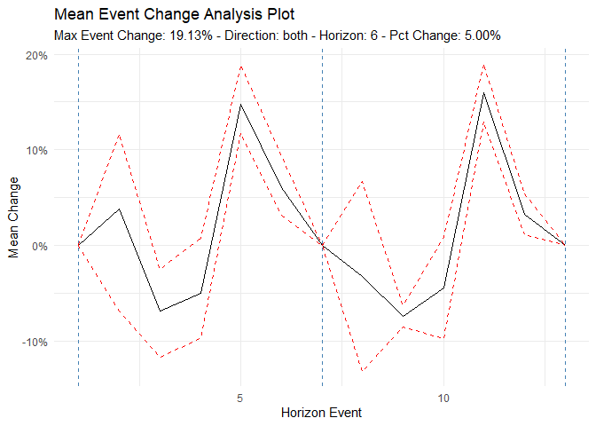
ts_time_event_analysis_tbl(
  .data = df,
  .horizon = 6,
  .date_col = date_col,
  .value_col = value,
  .direction = "both"
) %>%
  ts_event_analysis_plot(.plot_type = "individual")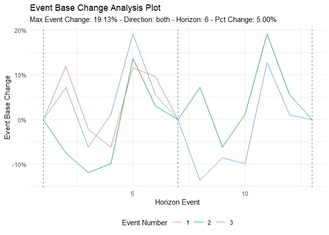
ARIMA Simulators
output <- ts_arima_simulator()
output$plots$static_plot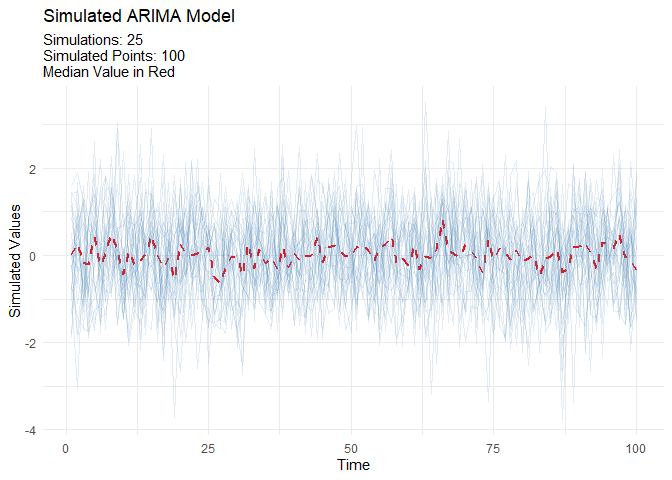
Automatic Workflows which can be thought of as Boiler Plate Time Series modeling. This is in it’s infancy in this package.
| Auto Workflows | Boilerplate Workflow |
|---|---|
| ts_auto_arima() | Boilerplate Workflow |
| ts_auto_arima_xgboost() | Boilerplate Workflow |
| ts_auto_croston() | Boilerplate Workflow |
| ts_auto_exp_smoothing() | Boilerplate Workflow |
| ts_auto_glmnet() | Boilerplate Workflow |
| ts_auto_lm() | Boilerplate Workflow |
| ts_auto_mars() | Boilerplate Workflow |
| ts_auto_nnetar() | Boilerplate Workflow |
| ts_auto_prophet_boost() | Boilerplate Workflow |
| ts_auto_prophet_reg() | Boilerplate Workflow |
| ts_auto_smooth_es() | Boilerplate Workflow |
| ts_auto_svm_poly() | Boilerplate Workflow |
| ts_auto_svm_rbf() | Boilerplate Workflow |
| ts_auto_theta() | Boilerplate Workflow |
| ts_auto_xgboost() | Boilerplate Workflow |
This is just a start of what is in this package!