Analyzing Time Series Growth with ts_growth_rate_vec() in healthyR.ts
rtip
healthyrts
timeseries
Author
Steven P. Sanderson II, MPH
Published
October 16, 2023
Introduction
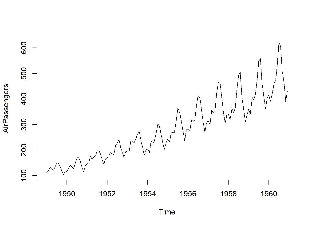
Time series data is essential for understanding trends and making forecasts in various fields, from finance to healthcare. Analyzing the growth rate of time series data is a crucial step in uncovering valuable insights. In the world of R programming, the healthyR.ts library introduces a powerful tool to calculate growth rates and log-differenced growth rates with the ts_growth_rate_vec() function. In this blog post, we’ll explore how this function works and how it can be used for effective time series analysis.
Understanding ts_growth_rate_vec():
The ts_growth_rate_vec() function is part of the healthyR.ts library, designed to work with numeric vectors or time series data. It calculates the growth rate or log-differenced growth rate of the provided data, offering valuable insights into the underlying trends and patterns.
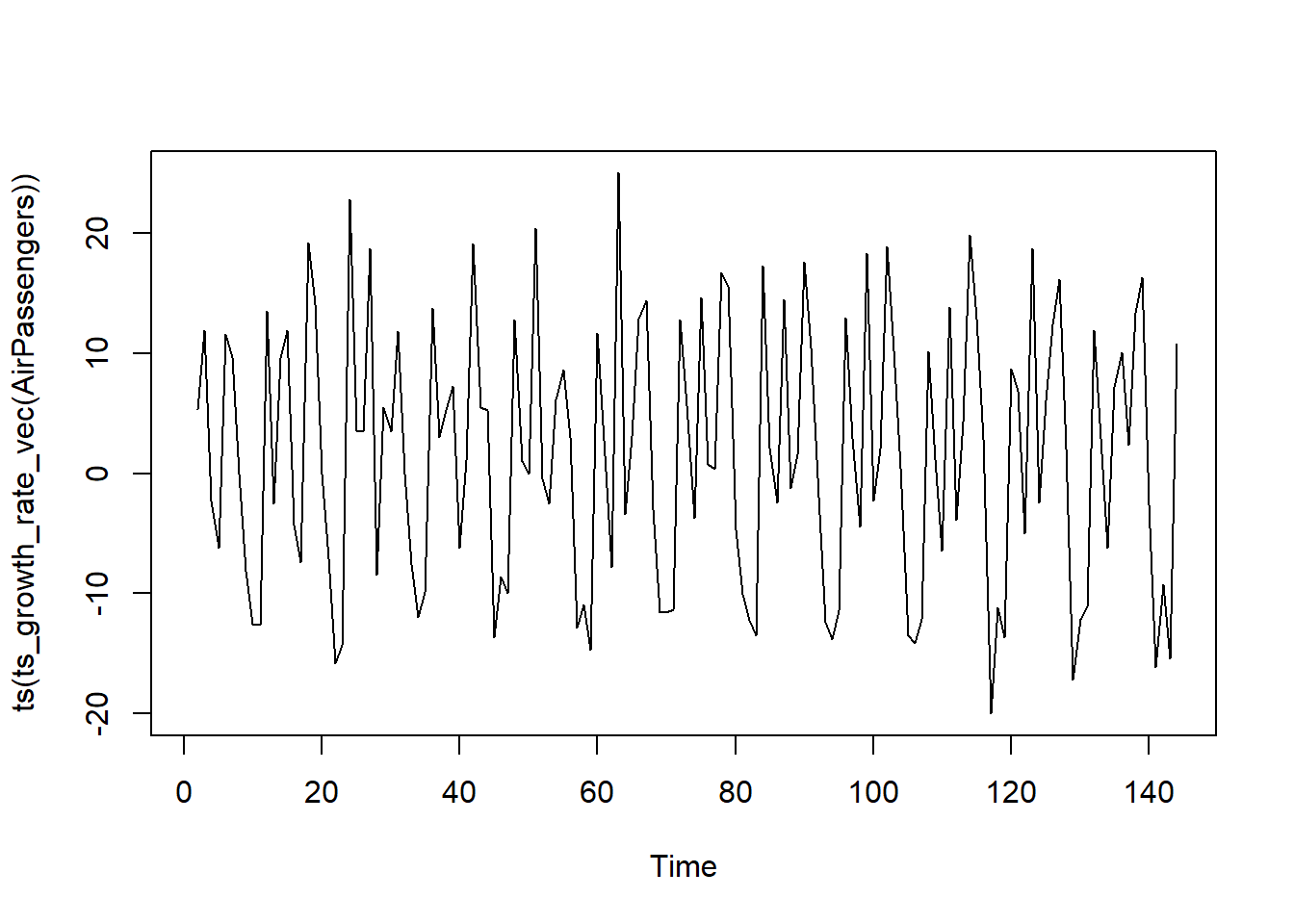
The output provides growth rates for the AirPassengers dataset. This basic calculation can help you understand how the data is evolving over time. The growth rates are calculated from one point to the next, giving you an idea of the speed at which the values are changing.
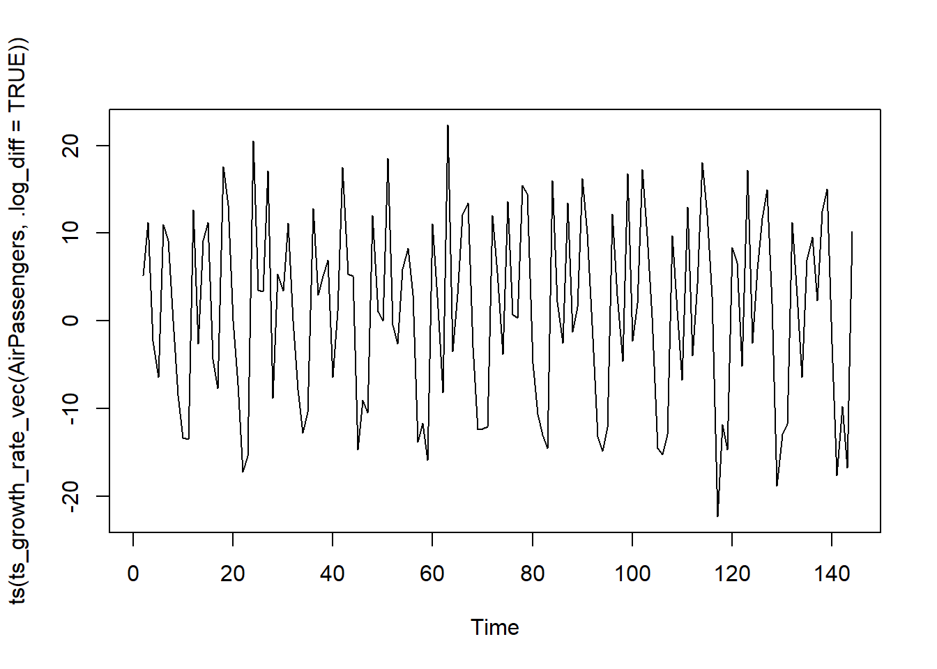
This example introduces the option to apply scaling and a power transformation. The resulting growth rates can help uncover trends that might not be apparent in the original data. Using a log-differenced growth rate is particularly useful for capturing the percentage change, making it easier to interpret the data.
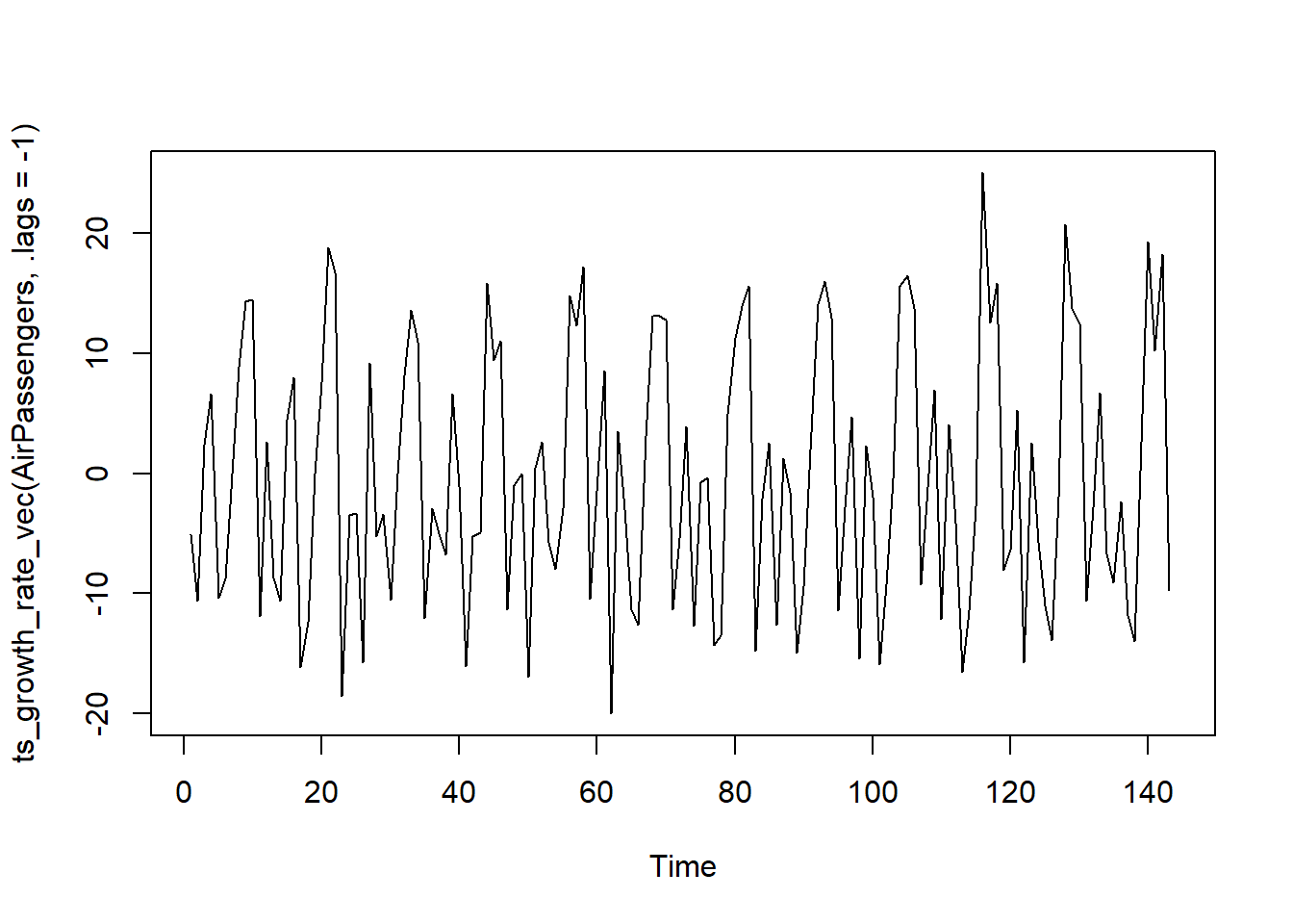
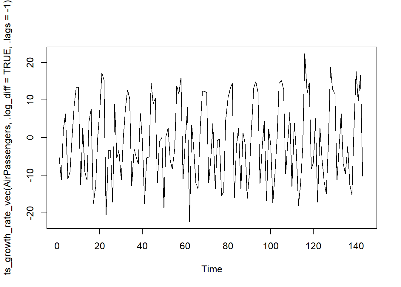
In this case, the function calculates the log differences of the time series with lags. This is helpful when you want to observe the changes between data points at different time intervals. It can reveal patterns that might not be apparent in the basic growth rate calculation.
This example combines all the mentioned features to provide a comprehensive analysis of the data. It’s a powerful way to understand how the growth rate is affected by various factors, such as scaling and time lags.
Conclusion:
The ts_growth_rate_vec() function in the healthyR.ts library is a versatile tool for time series analysis. Whether you need a basic growth rate, want to apply scaling and transformation, or work with lagged data, this function has you covered. It’s a valuable asset for R programmers, helping them uncover hidden insights within time series data.
Incorporating this function into your data analysis workflow can provide you with a deeper understanding of how values change over time. Whether you’re working with financial data, healthcare data, or any other time series dataset, ts_growth_rate_vec() is a powerful addition to your R programming toolkit. Start exploring your time series data today and discover the trends and patterns that lie within.