# Install and load the required libraries
# install.packages("splines")
library(splines)Introduction
Spline regression is particularly useful when the relationship between the independent and dependent variables is not adequately captured by a linear model. It involves fitting a piecewise continuous curve (spline) to the data. Let’s dive into the process using R.
Example
Step 1: Load the Necessary Libraries
Step 2: Generate Sample Data
For our example, let’s create a hypothetical dataset:
# Generate sample data
set.seed(123)
x <- seq(1, 10, length.out = 100)
y <- 3 * sin(x) + rnorm(100, mean = 0, sd = 0.5)
Step 3: Fit a Spline Regression Model
Now, let’s fit a spline regression model to our data:
# Fit a spline regression model
spline_model <- lm(y ~ ns(x, df = 4))
Here, ns from the splines package is used to create a natural spline basis with 4 degrees of freedom.
Step 4: Visualize the Results
Visualizing the data and the fitted spline is crucial for understanding the model’s performance:
# Visualize the data and fitted spline
plot(x, y, main = "Spline Regression Example", xlab = "X", ylab = "Y")
lines(x, predict(spline_model), col = "red", lwd = 2)
legend("topright", legend = "Fitted Spline", col = "red", lwd = 2)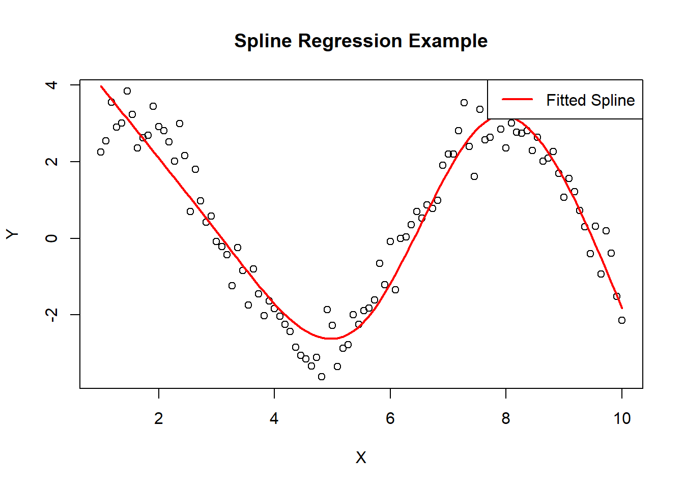
This code generates a plot with the original data points and overlays the fitted spline.
Step 5: Examine Residuals
Checking residuals helps assess the model’s goodness of fit:
# Examine residuals
residuals <- residuals(spline_model)
plot(x, residuals, main = "Residuals of Spline Regression", xlab = "X",
     ylab = "Residuals")
abline(h = 0, col = "red", lty = 2)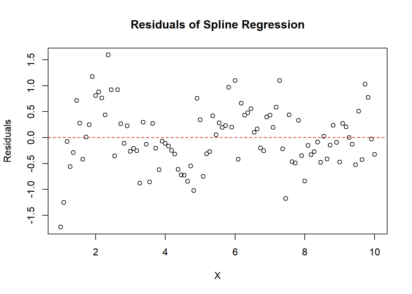
This plot shows the residuals (the differences between observed and predicted values) against the independent variable.
You Try!
Now that you’ve seen the basics, I encourage you to try spline regression on your own datasets. Experiment with different degrees of freedom (df parameter) in the ns function to observe how it affects the fit.
Remember, the power of spline regression lies in its ability to capture complex patterns in your data. Don’t hesitate to tweak the code and visualize the results to gain a deeper understanding.
Feel free to share your experiences or ask questions in the comments. Happy coding!
That wraps up our journey into spline regression in R. I hope you found this tutorial helpful and inspiring for your data analysis endeavors.