Introduction

There are two components to time-series clustering with {healthyR.ts}. There is the function that will create the clustering data along with a slew of other information and then there is a plotting function that will plot out the data in a time-series fashion colored by cluster.

The first function as mentioned is the function ts_feature_cluster(), and the next is ts_feature_cluster_plot()

Function Reference:

We are going to use the built-in AirPassengers data set for this example so let’s get right to it!

Library Load

suppressPackageStartupMessages(library(dplyr))
suppressPackageStartupMessages(library(healthyR.ts))

Data

Now that our libraries are loaded we can go ahead and get the data and run it through the function.

data_tbl <- ts_to_tbl(AirPassengers) %>%
  select(-index) %>%
  mutate(group_id = rep(1:12, 12))

output <- ts_feature_cluster(
  .data = data_tbl,
  .date_col = date_col,
  .value_col = value,
  group_id,
  .features = c("acf_features","entropy"),
  .scale = TRUE,
  .prefix = "ts_",
  .centers = 3
)

Registered S3 method overwritten by 'quantmod':
  method            from
  as.zoo.data.frame zoo

Now that we have our data and our output, lets first take a look at our data so we can see what we passed to it.

glimpse(data_tbl)

Rows: 144
Columns: 3
$ date_col <date> 1949-01-01, 1949-02-01, 1949-03-01, 1949-04-01, 1949-05-01, …
$ value    <dbl> 112, 118, 132, 129, 121, 135, 148, 148, 136, 119, 104, 118, 1…
$ group_id <int> 1, 2, 3, 4, 5, 6, 7, 8, 9, 10, 11, 12, 1, 2, 3, 4, 5, 6, 7, 8…

Now as mentioned, the output list contains many items. There are both data items and plot items.

First though, you will notice in the ts_feature_cluster() function that there is a parameter called .features, this allows you to pass in a list of quoted functions to apply to the time-series. This means that you can create a function your self in the .GlobalEnviron and pass that as a quoted argument to this parameter.

For example you could create your own function called my_mean. Let’s see how this would work.

my_mean <- function(x) ret <- mean(x, na.rm = TRUE) return(ret)

You can then call this by using .features = c("my_mean").

Pretty simple!

Under the hood this function itself makes use of timetk::tk_tsfeatures() which is a tidyverse compliant wrapper to tsfeatures::tsfeatures()

Here are the links to those functions:

Now let’s take a look at the output

Function Output

ts_feature_cluster()

As mentioned there are several outputs from the ts_feature_cluster(). Those are as follows:

Data Section

ts_feature_tbl
user_item_matrix_tbl
mapped_tbl
scree_data_tbl
input_data_tbl (the original data)

Plots

static_plot
plotly_plot

Now that we have our output, let’s take a look at each individual component of the output.

ts_feature_tbl

output$data$ts_feature_tbl |> glimpse()

Rows: 12
Columns: 8
$ group_id       <int> 1, 2, 3, 4, 5, 6, 7, 8, 9, 10, 11, 12
$ ts_x_acf1      <dbl> 0.7405485, 0.7301127, 0.7664718, 0.7151592, 0.7296932, …
$ ts_x_acf10     <dbl> 1.552193, 1.499645, 1.622249, 1.457441, 1.479361, 1.609…
$ ts_diff1_acf1  <dbl> -0.09954220, -0.01546920, -0.47063892, -0.25269676, -0.…
$ ts_diff1_acf10 <dbl> 0.4742052, 0.6538733, 0.5623693, 0.4570952, 0.4168840, …
$ ts_diff2_acf1  <dbl> -0.18227012, -0.14657790, -0.62033635, -0.55453480, -0.…
$ ts_seas_acf1   <dbl> 0.2829677, 0.2792932, 0.2947631, 0.2931678, 0.2888097, …
$ ts_entropy     <dbl> 0.4945771, 0.4818227, 0.6426700, 0.6798957, 0.8772866, …

user_item_matrix_tbl

output$data$user_item_matrix_tbl |> glimpse()

Rows: 12
Columns: 8
$ group_id       <int> 1, 2, 3, 4, 5, 6, 7, 8, 9, 10, 11, 12
$ ts_x_acf1      <dbl> 0.7405485, 0.7301127, 0.7664718, 0.7151592, 0.7296932, …
$ ts_x_acf10     <dbl> 1.552193, 1.499645, 1.622249, 1.457441, 1.479361, 1.609…
$ ts_diff1_acf1  <dbl> -0.09954220, -0.01546920, -0.47063892, -0.25269676, -0.…
$ ts_diff1_acf10 <dbl> 0.4742052, 0.6538733, 0.5623693, 0.4570952, 0.4168840, …
$ ts_diff2_acf1  <dbl> -0.18227012, -0.14657790, -0.62033635, -0.55453480, -0.…
$ ts_seas_acf1   <dbl> 0.2829677, 0.2792932, 0.2947631, 0.2931678, 0.2888097, …
$ ts_entropy     <dbl> 0.4945771, 0.4818227, 0.6426700, 0.6798957, 0.8772866, …

mapped_tbl

output$data$mapped_tbl |> glimpse()

Rows: 3
Columns: 3
$ centers <int> 1, 2, 3
$ k_means <list> [1, 1, 1, 1, 1, 1, 1, 1, 1, 1, 1, 1, 0.7416450, 1.5450677, -0.…
$ glance  <list> [<tbl_df[1 x 4]>], [<tbl_df[1 x 4]>], [<tbl_df[1 x 4]>]

scree_data_tbl

output$data$scree_data_tbl |> glimpse()

Rows: 3
Columns: 2
$ centers      <int> 1, 2, 3
$ tot.withinss <dbl> 1.8324477, 0.7364934, 0.4571258

input_data_tbl

output$data$input_data_tbl |> glimpse()

Rows: 144
Columns: 3
$ date_col <date> 1949-01-01, 1949-02-01, 1949-03-01, 1949-04-01, 1949-05-01, …
$ value    <dbl> 112, 118, 132, 129, 121, 135, 148, 148, 136, 119, 104, 118, 1…
$ group_id <int> 1, 2, 3, 4, 5, 6, 7, 8, 9, 10, 11, 12, 1, 2, 3, 4, 5, 6, 7, 8…

Now the plots.

static_plot

output$plots$static_plot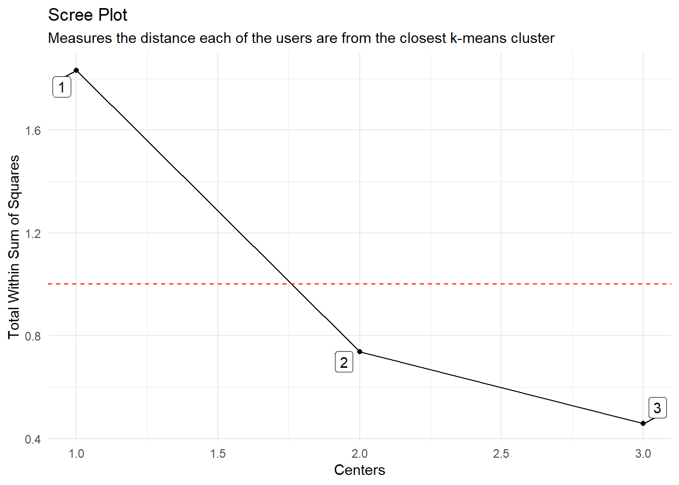

plotly_plot

output$plots$plotly_plot

Now that we have seen the output of the ts_feature_cluster() function, let’s take a look at the output of the ts_feature_cluster_plot() function.

ts_feature_cluster_plot()

This function itself returns a list object of a multitude of data. First before we get into that lets look at the function call itself:

ts_feature_cluster_plot(
  .data,
  .date_col,
  .value_col,
  ...,
  .center = 3,
  .facet_ncol = 3,
  .smooth = FALSE
)

The data that comes back from this function is:

Data Section

original_data
kmm_data_tbl
user_item_tbl
cluster_tbl

Plots

static_plot
plotly_plot

K-Means Object

k-means object

We will go through the same exercise and show the output of all the sections. First we have to create the output. The static plot will automatically print out.

plot_out <- ts_feature_cluster_plot(
  .data = output,
  .date_col = date_col,
  .value_col = value,
  .center = 2,
  group_id
)

Joining, by = "group_id"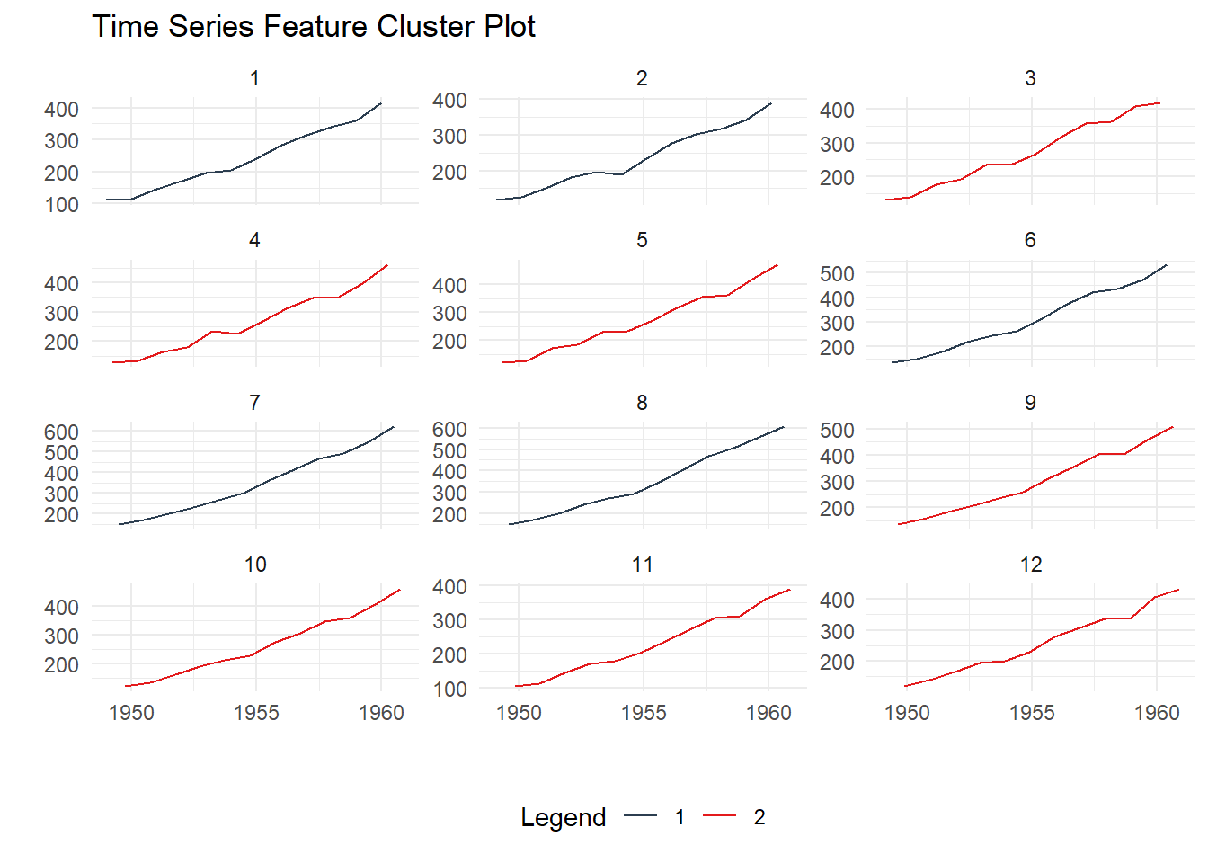

The Data Section:

original_data

plot_out$data$original_data |> glimpse()

Rows: 144
Columns: 3
$ date_col <date> 1949-01-01, 1949-02-01, 1949-03-01, 1949-04-01, 1949-05-01, …
$ value    <dbl> 112, 118, 132, 129, 121, 135, 148, 148, 136, 119, 104, 118, 1…
$ group_id <int> 1, 2, 3, 4, 5, 6, 7, 8, 9, 10, 11, 12, 1, 2, 3, 4, 5, 6, 7, 8…

kmm_data_tbl

plot_out$data$kmm_data_tbl |> glimpse()

Rows: 3
Columns: 3
$ centers <int> 1, 2, 3
$ k_means <list> [1, 1, 1, 1, 1, 1, 1, 1, 1, 1, 1, 1, 0.7416450, 1.5450677, -0.…
$ glance  <list> [<tbl_df[1 x 4]>], [<tbl_df[1 x 4]>], [<tbl_df[1 x 4]>]

user_item_data

plot_out$data$user_item_data |> glimpse()

 NULL

cluster_tbl

plot_out$data$cluster_tbl |> glimpse()

Rows: 12
Columns: 9
$ cluster        <int> 1, 1, 2, 2, 2, 1, 1, 1, 2, 2, 2, 2
$ group_id       <int> 1, 2, 3, 4, 5, 6, 7, 8, 9, 10, 11, 12
$ ts_x_acf1      <dbl> 0.7405485, 0.7301127, 0.7664718, 0.7151592, 0.7296932, …
$ ts_x_acf10     <dbl> 1.552193, 1.499645, 1.622249, 1.457441, 1.479361, 1.609…
$ ts_diff1_acf1  <dbl> -0.09954220, -0.01546920, -0.47063892, -0.25269676, -0.…
$ ts_diff1_acf10 <dbl> 0.4742052, 0.6538733, 0.5623693, 0.4570952, 0.4168840, …
$ ts_diff2_acf1  <dbl> -0.18227012, -0.14657790, -0.62033635, -0.55453480, -0.…
$ ts_seas_acf1   <dbl> 0.2829677, 0.2792932, 0.2947631, 0.2931678, 0.2888097, …
$ ts_entropy     <dbl> 0.4945771, 0.4818227, 0.6426700, 0.6798957, 0.8772866, …

The plot data.

static_plot

plot_out$plot$static_plot

plotly_plot

plot_out$plot$plotly_plot

The K-Means Object

kmeans_object

plot_out$kmeans_object

[[1]]
K-means clustering with 2 clusters of sizes 5, 7

Cluster means:
  ts_x_acf1 ts_x_acf10 ts_diff1_acf1 ts_diff1_acf10 ts_diff2_acf1 ts_seas_acf1
1 0.7456468   1.568532     0.1172685      0.4858013    -0.1799728    0.2876449
2 0.7387865   1.528308    -0.2909349      0.3638392    -0.5916245    0.2930543
  ts_entropy
1  0.4918321
2  0.6438176

Clustering vector:
 [1] 1 1 2 2 2 1 1 1 2 2 2 2

Within cluster sum of squares by cluster:
[1] 0.3704304 0.3660630
 (between_SS / total_SS =  59.8 %)

Available components:

[1] "cluster"      "centers"      "totss"        "withinss"     "tot.withinss"
[6] "betweenss"    "size"         "iter"         "ifault"

Thanks for reading!