Introduction

Random walks are a type of stochastic process that can be used to model the movement of a particle or system over time. At each time step, the position of the particle is updated based on a random step drawn from a given probability distribution. This process can be represented as a sequence of independent and identically distributed (i.i.d.) random variables, and the resulting path traced by the particle is known as a random walk.

Random walks have a wide range of applications, including modeling the movement of stock prices, animal migration, and the spread of infectious diseases. They are also a fundamental concept in probability and statistics, and have been studied extensively in the literature.

The {TidyDensity} package provides a convenient way to generate and visualize random walks using the tidy_random_walk() function. This function takes a probability distribution as an argument, and generates a random walk by sampling from this distribution at each time step. For example, to generate a random walk with normally distributed steps, we can use the tidy_normal() function as follows:

library(TidyDensity)

# Generate a random walk with normally distributed steps
rw <- tidy_random_walk(tidy_normal())

The resulting object rw is a tibble with the typical tidy_ distribution columns and one augmented column called random_walk_value. The columns that are output are:

sim_number The current simulation number from the tidy_ distribution
x (You can think of this as time t)
y The randomly generated value.
dx & dy The density estimates of y at x
p & q The probability and quantile values of y
random_walk_value The random walk value generated from tidy_random_walk() (You can think of this as the position of the particle at time t or the x)

To visualize the random walk, we can use the tidy_random_walk_autoplot() function, which creates a ggplot object showing the position of the particle at each time step. For example:

# Visualize the random walk
tidy_random_walk_autoplot(rw)

This will produce a plot showing the trajectory of the particle over time. You can customize the appearance of the plot by passing additional arguments to the tidy_random_walk_autoplot() function, such as the geom argument to specify the type of plot to use (e.g. geom = “line” for a line plot, or geom = “point” for a scatter plot).

In summary, the {TidyDensity} package provides a convenient and user-friendly interface for generating and visualizing random walks. With the tidy_random_walk() and tidy_random_walk_autoplot() functions, you can easily explore the behavior of random walks and their applications in a wide range of contexts.

Let’s take a look at these functions.

Function

Firstly we will look at the tidy_random_walk() function.

tidy_random_walk(
  .data,
  .initial_value = 0,
  .sample = FALSE,
  .replace = FALSE,
  .value_type = "cum_prod"
)

Here are the arguments that get provided to the parameters of this function.

.data - The data that is being passed from a tidy_ distribution function.
.initial_value - The default is 0, this can be set to whatever you want.
.sample - This is a boolean value TRUE/FALSE. The default is FALSE. If set to TRUE then the y value from the tidy_ distribution function is sampled.
.replace - This is a boolean value TRUE/FALSE. The default is FALSE. If set to TRUE AND .sample is set to TRUE then the replace parameter of the sample function will be set to TRUE.
.value_type - This can take one of three different values for now. These are the following:
- “cum_prod” - This will take the cumprod of y
- “cum_sum” - This will take the cumsum of y

Now let’s do the same with the tidy_random_walk_autoplot() function.

tidy_random_walk_autoplot(
  .data,
  .line_size = 1,
  .geom_rug = FALSE,
  .geom_smooth = FALSE,
  .interactive = FALSE
)

Here are the arguments that get provided to the parameters.

.data - The data passed in from a tidy_distribution function like tidy_normal()
.line_size - The size param ggplot
.geom_rug - A Boolean value of TRUE/FALSE, FALSE is the default. TRUE will return the use of ggplot2::geom_rug()
.geom_smooth - A Boolean value of TRUE/FALSE, FALSE is the default. TRUE will return the use of ggplot2::geom_smooth() The aes parameter of group is set to FALSE. This ensures a single smoothing band returned with SE also set to FALSE. Color is set to ‘black’ and linetype is ‘dashed’.
.interactive - A Boolean value of TRUE/FALSE, FALSE is the default. TRUE will return an interactive plotly plot.

Examples

Let’s go over some examples.

library(TidyDensity)

dist_data <- tidy_normal(.sd = .1, .num_sims = 5)

tidy_random_walk(.data = dist_data, .value_type = "cum_sum") %>%
  tidy_random_walk_autoplot()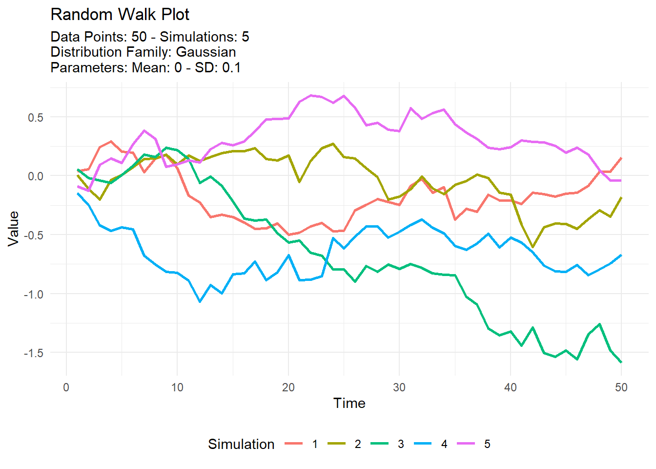

And another.

tidy_normal(.sd = .1, .num_sims = 20) %>%
  tidy_random_walk(
    .value_type = "cum_sum", 
    .sample = TRUE, 
    .replace = TRUE
    ) %>%
  tidy_random_walk_autoplot()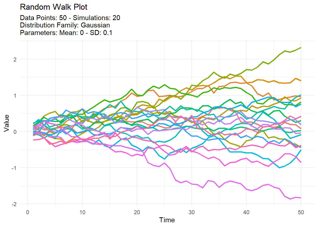

Now let’s get an interactive one.

tidy_normal(.sd = .1, .num_sims = 20) %>%
  tidy_random_walk(
    .value_type = "cum_sum", 
    .sample = TRUE, 
    .replace = TRUE
    ) %>%
  tidy_random_walk_autoplot(.interactive = TRUE)

One last example, let’s use a different distribution. Let’s use a cauchy distribution.

tidy_cauchy(.num_sims = 9, .location = .5) %>%
  tidy_random_walk(.value_type = "cum_sum", .sample = TRUE) %>%
  tidy_random_walk_autoplot()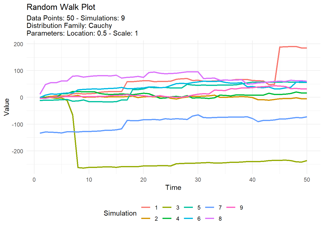

Voila!