Introduction

Histogram binning is a technique used in data visualization to group continuous data into a set of discrete bins, or intervals. The purpose of histogram binning is to represent the distribution of a dataset in a graphical format, allowing for easy identification of patterns and outliers. However, there are several challenges that can arise when working with histogram binning.

One major challenge is determining the appropriate number of bins to use. If there are too few bins, the histogram may not accurately represent the underlying distribution of the data. On the other hand, if there are too many bins, the histogram may become cluttered and difficult to interpret. To overcome this challenge, there are several strategies that can be employed, such as the Scott’s normal reference rule, Freedman-Diaconis rule, or the Rice rule, to determine the optimal number of bins.

Another challenge with histogram binning is dealing with outliers. If a dataset has outliers, they can greatly skew the distribution of the data and make it difficult to interpret the histogram. One strategy to handle outliers is to use a log-scale on the x-axis, which can help to reduce their impact on the histogram. Alternatively, one could remove the outlier data points before creating the histogram.

A further challenge is to choose the width of the bin that best represents the data. Too narrow bins might cause overfitting and too wide bins may cause loss of information. Different widths of bin can lead to a different representation of the data and hence a different conclusion. To overcome this, one could use the Freedman-Diaconis rule which take into consideration the range and the size of the sample to provide a robust and adaptive way to choose the width of the bin

A simple solution to these challenges is the opt_bin() function in the {healthyR} library for R. This function uses an optimal binning algorithm to automatically determine the number of bins and bin widths that best represent the data. This can save a lot of time and effort when working with histograms and can help to ensure that the resulting histograms are accurate and easy to interpret.

In conclusion, histogram binning is a useful technique for visualizing the distribution of data, but it can be challenging to determine the appropriate number of bins and bin widths. Strategies such as Scott’s normal reference rule, Freedman-Diaconis rule, or the Rice rule can be used to determine the optimal number of bins. Outliers and bin width selection also can be challenges to take into account, and a function such as opt_bin() in the {healthyR} library can be used to overcome these challenges and create high-quality histograms with ease.

Function

Here is the full call.

opt_bin(.data, .value_col, .iters = 30)

Here are the arguments that get passed to the parameters.

.data - The data set in question
.value_col - The column that holds the values
.iters - How many times the cost function loop should run

Now under I will provide some code and it’s explanation under the hood that exaplains how this works.

Here is a breakdown of what each part of the code is doing:

n <- 2:iters: this line creates a sequence of numbers starting at 2 and ending at the number specified by the variable “iters”
c <- base::numeric(base::length(n)) and d <- c: These lines create two empty numeric vectors (arrays) called “c” and “d” with the same length as the sequence “n”
for (i in 1:length(n)) {...}: This is a for loop that iterates through each number in the sequence “n”
d[i] <- diff(range( data ) ) / n[i]: Inside the loop, this line calculates the width of the bin for the current iteration by dividing the range of the data by the current number in the sequence “n”
hp <- graphics::hist(data, breaks = edges, plot = FALSE) and ki <- hp$counts: This creates a histogram of the data using the current bin width and then gets the count of data points in each bin
k <- mean(ki) and v <- sum((ki-k)^2/n[i]): this line uses the counts from the previous step to calculate the average count across all bins (k) and the variance of the counts across all bins (v)
c[i] <- (2*k - v)/d[i]^2: this line calculates the cost function for the current bin width, which is based on k and v
idx <- which.min(c) and opt_d <- d[idx]: this line finds the index in the “c” vector where the cost function is the lowest and stores that value in the variable “idx”
edges <- seq(min(data), max(data), length = n[idx]) and edges <- tibble::as_tibble(edges): this line creates a new sequence of numbers representing the edges of the bins with the optimal bin width
return(edges): this line returns the sequence of optimal bin edges that the function has determined

Overall, this function will return an optimal set of bin edges for a histogram of the given data, the function uses an iterative process and consider the balance between the number of bins and the width of the bins to find the optimal width of the bins for the histogram. This could save a lot of time and effort for the data analysts as it can help to ensure that the resulting histograms are accurate and easy to interpret.

Example

Let’s look at some examples.

library(healthyR)
library(tidyverse)

df_tbl <- rnorm(n = 1000, mean = 0, sd = 1)
df_tbl <- df_tbl %>%
  as_tibble()

opt_bin(
  .data = df_tbl,
  .value_col = value
  , .iters = 100
)

# A tibble: 6 × 1
   value
   <dbl>
1 -3.04 
2 -1.81 
3 -0.585
4  0.644
5  1.87 
6  3.10

Now lets user a smaller n to see how the output changes

opt_bin(
  .data = as_tibble(rnorm(n = 50)),
  value,
  100
)

# A tibble: 11 × 1
     value
     <dbl>
 1 -1.69  
 2 -1.24  
 3 -0.797 
 4 -0.351 
 5  0.0944
 6  0.540 
 7  0.986 
 8  1.43  
 9  1.88  
10  2.32  
11  2.77

Let’s visualize.

rn <- rnorm(50)
hist(rn)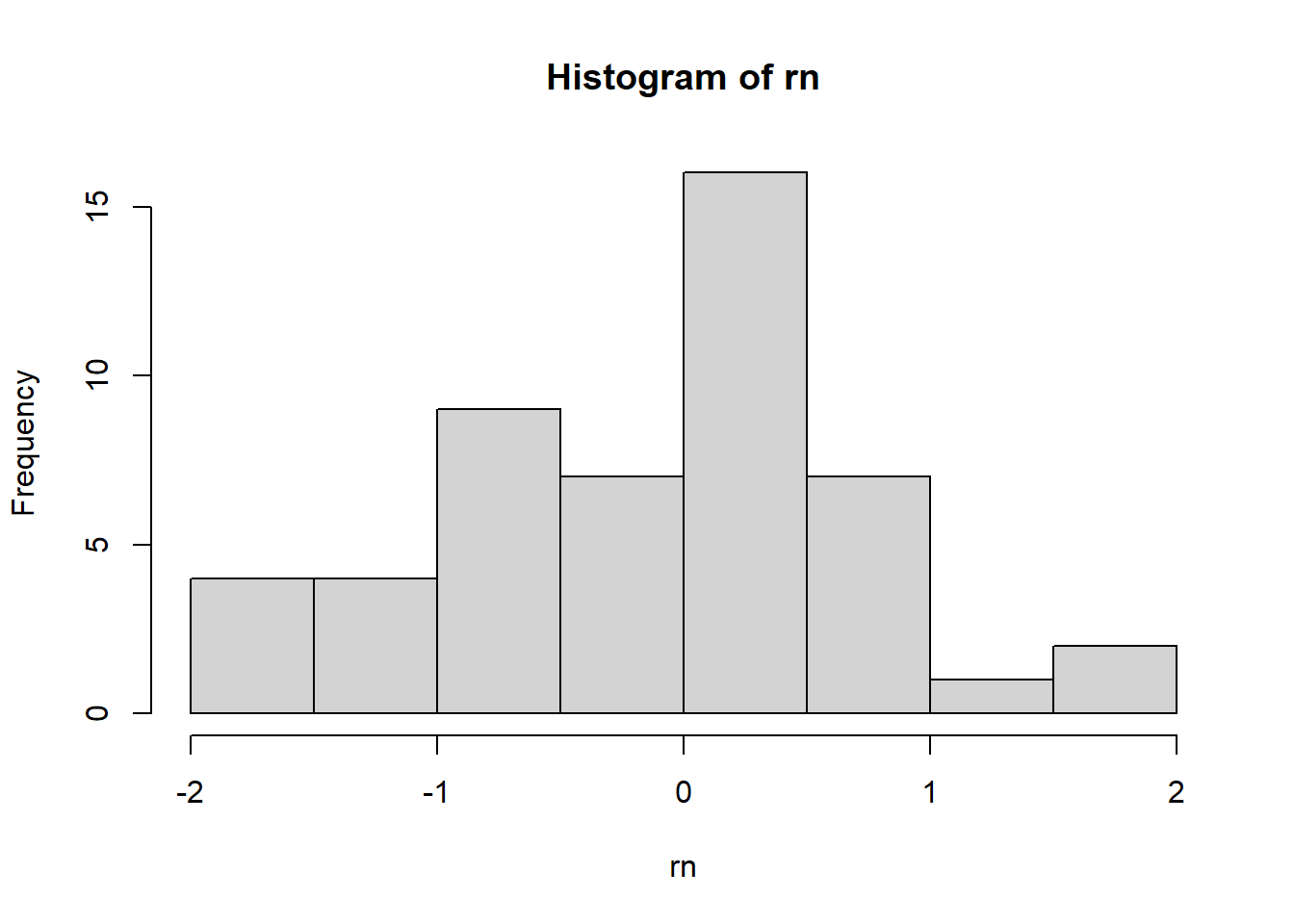

Now let’s use opt_bin()

hist(rn, breaks = opt_bin(as_tibble(rn), value) %>% pull())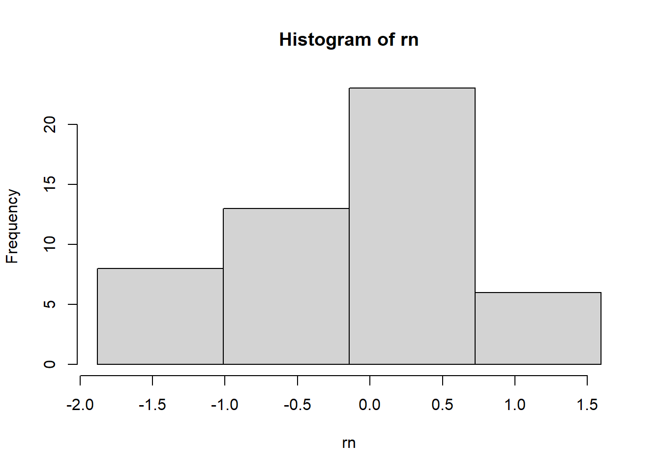

Voila!