Introduction

Time series analysis is a crucial tool for forecasting and understanding trends in various industries, including finance, economics, and engineering. However, traditional time series analysis methods can be limiting, and they may not always capture the complex dynamics of real-world data. That’s where the R package {healthyR.ts} comes in.

The {healthyR.ts} package is a powerful tool for time series analysis that offers a wide range of functions for cleaning, transforming, and analyzing time series data. One of its standout features is the ts_brownian_motion_augment() function, which allows you to add a brownian motion to a given time series dataset. This powerful tool can be used to simulate more realistic and complex scenarios, making it an invaluable tool for forecasters and data analysts.

Brownian motion is a random walk process that can be used to model the movement of particles in a fluid. It has been widely used in mathematical finance, physics, and engineering to model the random movements of stock prices, pollutant concentrations, and other phenomena. By adding a brownian motion to a time series dataset, the ts_brownian_motion_augment() function allows users to capture the unpredictable and random nature of real-world data, making time series analysis more accurate and reliable.

The ts_brownian_motion_augment() function is easy to use and requires no prior knowledge of brownian motion or advanced mathematics. With just a few lines of code, users can quickly add a brownian motion to their time series dataset and begin analyzing the data with greater precision and confidence.

This set of functionality will be included in the next release which will be coming soon as it also speeds up the current ts_brownian_motion() function by 49x!

Function

Here is the full function call.

ts_brownian_motion_augment(
  .data,
  .date_col,
  .value_col,
  .time = 100,
  .num_sims = 10,
  .delta_time = NULL
)

Let’s take a look at the arguments for the parameters.

.data - The data.frame/tibble being augmented.
.date_col - The column that holds the date.
.value_col - The value that is going to get augmented. The last value of this column becomes the initial value internally.
.time - How many time steps ahead.
.num_sims - How many simulations should be run.
.delta_time - Time step size.

Example

Now for an example.

library(tidyquant)
library(dplyr)
library(timetk)
library(ggplot2)
library(healthyR.ts)

df <- FANG %>%
  filter(symbol == "FB") %>%
  select(symbol, date, adjusted) %>%
  filter_by_time(.date_var = date, .start_date = "2016-01-01") %>%
  tq_mutate(select = adjusted, mutate_fun = periodReturn,
            period = "daily", type = "log",
            col_rename = "daily_returns")

Let’s take a look at our initial data.

df

# A tibble: 252 × 4
   symbol date       adjusted daily_returns
   <chr>  <date>        <dbl>         <dbl>
 1 FB     2016-01-04    102.        0      
 2 FB     2016-01-05    103.        0.00498
 3 FB     2016-01-06    103.        0.00233
 4 FB     2016-01-07     97.9      -0.0503 
 5 FB     2016-01-08     97.3      -0.00604
 6 FB     2016-01-11     97.5       0.00185
 7 FB     2016-01-12     99.4       0.0189 
 8 FB     2016-01-13     95.4      -0.0404 
 9 FB     2016-01-14     98.4       0.0302 
10 FB     2016-01-15     95.0      -0.0352 
# … with 242 more rows

Now let’s augment it with the brownian motion and see that data set before we visualize it.

df %>%
  ts_brownian_motion_augment(
    .date_col = date,
    .num_sims = 50,
    .value_col = daily_returns,
    .delta_time = 0.00005
  )

# A tibble: 5,302 × 3
   sim_number  date       daily_returns
   <fct>       <date>             <dbl>
 1 actual_data 2016-01-04       0      
 2 actual_data 2016-01-05       0.00498
 3 actual_data 2016-01-06       0.00233
 4 actual_data 2016-01-07      -0.0503 
 5 actual_data 2016-01-08      -0.00604
 6 actual_data 2016-01-11       0.00185
 7 actual_data 2016-01-12       0.0189 
 8 actual_data 2016-01-13      -0.0404 
 9 actual_data 2016-01-14       0.0302 
10 actual_data 2016-01-15      -0.0352 
# … with 5,292 more rows

As you see the function preserves the names of the input columns!

Now, let’s see it!

df %>%
  ts_brownian_motion_augment(
    .date_col = date,
    .num_sims = 50,
    .value_col = daily_returns,
    .delta_time = 0.00005
  ) %>%
  ggplot(aes(x = date, y = daily_returns
             , group = sim_number, color = sim_number)) +
  geom_line() +
  theme_minimal() +
  theme(legend.position = "none") +
  labs(
    title = "FB Log Daily Returns for 2016",
    x = "Date",
    y = "Log Daily Returns"
  )

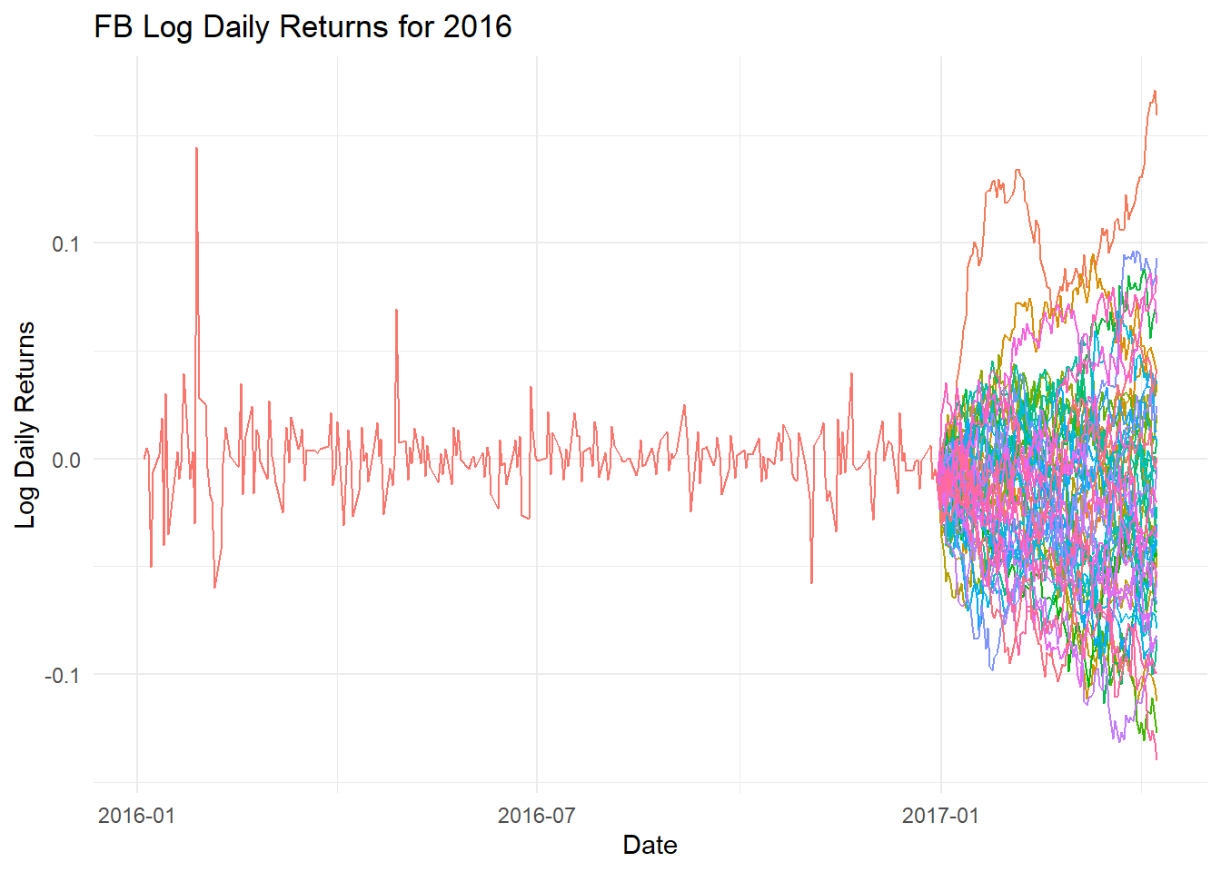
Voila!