Introduction

Geometric Brownian motion (GBM) is a widely used model in financial analysis for modeling the behavior of stock prices. It is a stochastic process that describes the evolution of a stock price over time, assuming that the stock price follows a random walk with a drift term and a volatility term.

One of the advantages of GBM is that it can capture the randomness and volatility of stock prices, which is a key feature of financial markets. GBM can also be used to estimate the expected return and volatility of a stock, which are important inputs for financial decision making.

Another advantage of GBM is that it can be used to generate simulations of future stock prices. These simulations can be used to estimate the probability of different outcomes, such as the probability of a stock price reaching a certain level in the future. This can be useful for risk management and for evaluating investment strategies.

GBM is also very easy to implement, making it a popular choice among financial analysts and traders.

The equation for GBM is: \[ dS(t) = μS(t)dt + σS(t)dW(t) \] Where:

\(dS(t)\) is the change in the stock price at time \(t\)

\(S(t)\) is the stock price at time \(t\)

\(μ\) is the expected return of the stock

\(σ\) is the volatility of the stock

\(dW(t)\) is a Wiener process (a random variable that describes the rate of change of a random variable over time)

It’s important to keep in mind that GBM is a model and not always a perfect fit to real-world stock prices. However, it’s a widely accepted model due to its capability to captures the key characteristics of stock prices and its mathematical tractability.

Attention R users! Are you looking for a reliable and accurate way to model stock prices? We have some exciting news for you! The next release of the R package {healthyR.ts} will include a new function, ts_geometric_brownian_motion(). This powerful function utilizes the geometric Brownian motion model to simulate stock prices, providing you with valuable insights and predictions for your financial analysis.

Function

Let’s take a look at the full function call.

ts_geometric_brownian_motion(
  .num_sims = 100,
  .time = 25,
  .mean = 0,
  .sigma = 0.1,
  .initial_value = 100,
  .delta_time = 1/365,
  .return_tibble = TRUE
)

Now let’s go over the arguments to the parameters.

.num_sims - Total number of simulations.
.time - Total time of the simulation.
.mean - Expected return
.sigma - Volatility
.initial_value - Integer representing the initial value.
.delta_time - Time step size.
.return_tibble The default is TRUE. If set to FALSE then an object of class matrix will be returned.

Example

Let’s go over a few examples.

library(healthyR.ts)

ts_geometric_brownian_motion()

# A tibble: 2,600 × 3
   sim_number        t     y
   <fct>         <int> <dbl>
 1 sim_number 1      1   100
 2 sim_number 2      1   100
 3 sim_number 3      1   100
 4 sim_number 4      1   100
 5 sim_number 5      1   100
 6 sim_number 6      1   100
 7 sim_number 7      1   100
 8 sim_number 8      1   100
 9 sim_number 9      1   100
10 sim_number 10     1   100
# … with 2,590 more rows

Now without returning a tibble object.

ts_geometric_brownian_motion(.num_sims = 5, .return_tibble = FALSE)

      sim_number 1 sim_number 2 sim_number 3 sim_number 4 sim_number 5
 [1,]    100.00000     100.0000    100.00000    100.00000     100.0000
 [2,]    101.04170     100.6583    100.46420     99.68513     100.3776
 [3,]    101.58155     100.8959    100.03621     98.91656     101.5732
 [4,]    100.91680     100.7494     99.47735     98.57117     101.1525
 [5,]     99.96787     101.3298     98.70899     99.03101     101.1557
 [6,]     99.29069     101.4187     98.32176     98.33018     101.5584
 [7,]     99.40451     101.5124     98.26237     97.79356     101.4934
 [8,]     99.35345     101.0328     98.69587     97.46604     101.9630
 [9,]     97.94177     100.9534     98.32630     96.95231     102.1643
[10,]     97.95812     101.3813     98.36934     96.64048     101.8546
[11,]     98.47820     101.8262     98.21492     96.12851     102.5529
[12,]     99.53016     102.5522     97.92270     95.97443     102.8912
[13,]     98.82850     102.7482     96.66348     96.26008     103.1899
[14,]     99.87335     102.9351     96.69635     96.15058     103.9259
[15,]    101.03605     103.3796     96.60162     96.63562     103.3790
[16,]    101.83475     103.1900     97.63875     96.00162     103.0422
[17,]    102.10155     103.5851     97.12873     95.99579     103.0913
[18,]    102.16085     103.2966     96.26772     95.95174     103.7034
[19,]    102.35736     103.7429     96.37355     96.02805     102.8406
[20,]    102.49297     104.5301     96.44318     96.28293     103.3507
[21,]    102.36953     105.1809     96.87639     97.32625     104.0307
[22,]    103.30672     104.7480     96.90017     97.16507     104.0751
[23,]    103.55433     104.9848     97.40063     97.49375     102.6901
[24,]    103.44429     104.3553     97.35982     97.39390     102.8163
[25,]    103.23952     102.9840     97.30287     97.66737     103.2160
[26,]    103.48365     103.6117     97.96290     97.91773     103.0579
attr(,".time")
[1] 25
attr(,".num_sims")
[1] 5
attr(,".mean")
[1] 0
attr(,".sigma")
[1] 0.1
attr(,".initial_value")
[1] 100
attr(,".delta_time")
[1] 0.002739726
attr(,".return_tibble")
[1] FALSE

Let’s visualize the GBM at different levels of volatility.

library(dplyr)
library(ggplot2)

gbm <- rbind(
  ts_geometric_brownian_motion(.sigma = 0.05) %>%
    mutate(volatility = as.factor("A) Sigma = 5%")),
  ts_geometric_brownian_motion(.sigma = 0.1) %>%
    mutate(volatility = as.factor("B) Sigma = 10%")),
  ts_geometric_brownian_motion(.sigma = .15) %>%
    mutate(volatility = as.factor("C) Sigma = 15%")),
  ts_geometric_brownian_motion(.sigma = .2) %>%
    mutate(volatility = as.factor("D) Sigma = 20%"))
)

gbm %>%
  ggplot(aes(x = t, y = y, group = sim_number, color = sim_number)) + 
  facet_wrap(~ volatility, scales = "free") +
  geom_line() +
  theme_minimal() +
  theme(legend.position = "none")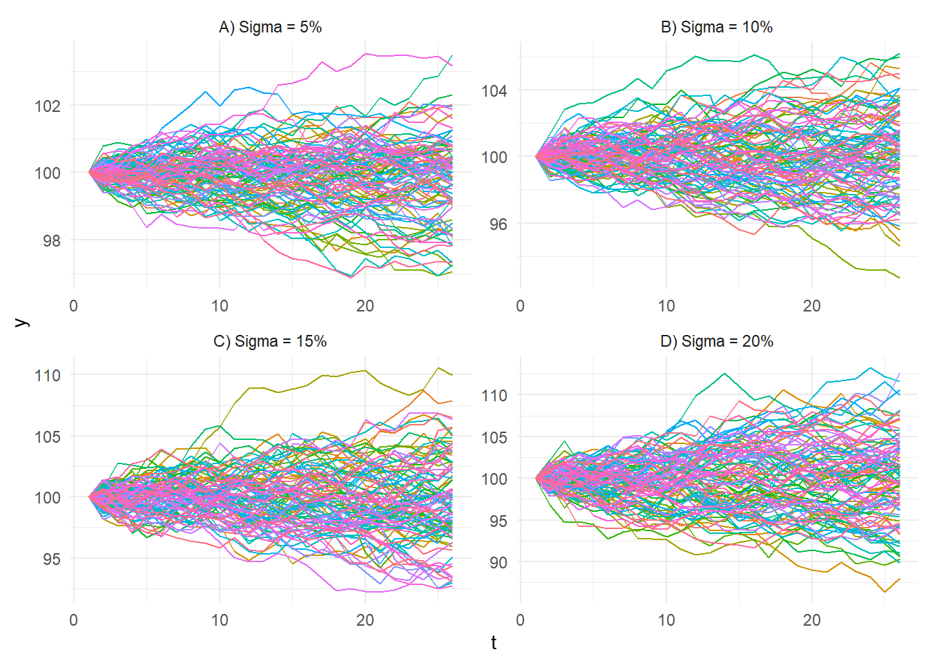

Voila!