Introduction

Brownian motion, also known as the random motion of particles suspended in a fluid, is a phenomenon that was first described by Scottish botanist Robert Brown in 1827. It occurs when a particle is subjected to a series of random collisions with the molecules in the fluid.

The motion of the particle can be described mathematically using the following equation:

\[ \frac{dx_t}{dt} = \mu + \sigma \cdot W_t \]

Where \(x_t\) represents the position of the particle at time t, \(\mu\) is the drift coefficient, \(\sigma\) is the diffusion coefficient, and \(W_t\) is a Wiener process (a type of random process).

Brownian motion has a number of important applications, including in the field of finance. It is used to model the random movements of financial assets, such as stocks, over time. It can also be used to estimate the volatility of an asset, as well as to calculate the prices of financial derivatives such as options.

In physics, Brownian motion is used to study the behavior of small particles suspended in a fluid, as well as to understand the properties of fluids at the molecular level. It has also been used to study the motion of biological molecules, such as proteins, within cells.

Overall, Brownian motion is a fundamental concept that has wide-ranging applications in a variety of fields, including finance, physics, and biology.

Function

Let’s take a look at a function to produce such results. This type of functionality will be coming to my R packages {TidyDensity} and to {healthyR.ts}

library(dplyr)


Attaching package: 'dplyr'

The following objects are masked from 'package:stats':

    filter, lag

The following objects are masked from 'package:base':

    intersect, setdiff, setequal, union

library(ggplot2)

Warning: package 'ggplot2' was built under R version 4.2.2

library(forcats)

brownian_motion <- function(T, N, delta_t) {
  # T: total time of the simulation (in seconds)
  # N: number of simulations to generate
  # delta_t: time step size (in seconds)
  
  # Initialize empty data.frame to store the simulations
  sim_data <- data.frame()
  
  # Generate N simulations
  for (i in 1:N) {
    # Initialize the current simulation with a starting value of 0
    sim <- c(0)
    
    # Generate the brownian motion values for each time step
    for (t in 1:(T / delta_t)) {
      sim <- c(sim, sim[t] + rnorm(1, mean = 0, sd = sqrt(delta_t)))
    }
    
    # Bind the time steps, simulation values, and simulation number together
    # in a data.frame and add it to the result
    sim_data <- rbind(
      sim_data, 
      data.frame(
        t = seq(0, T, delta_t), 
        y = sim, 
        sim_number = i
        )
      ) %>%
      as_tibble()
  }
  
  sim_data <- sim_data %>%
    mutate(sim_number = as_factor(sim_number)
                  )
  return(sim_data)
}

We see that the internal variable sim is set to 0, this in the future will be set to an initial value that a user can provide.

Examples

Let’s take a look at a couple of examples.

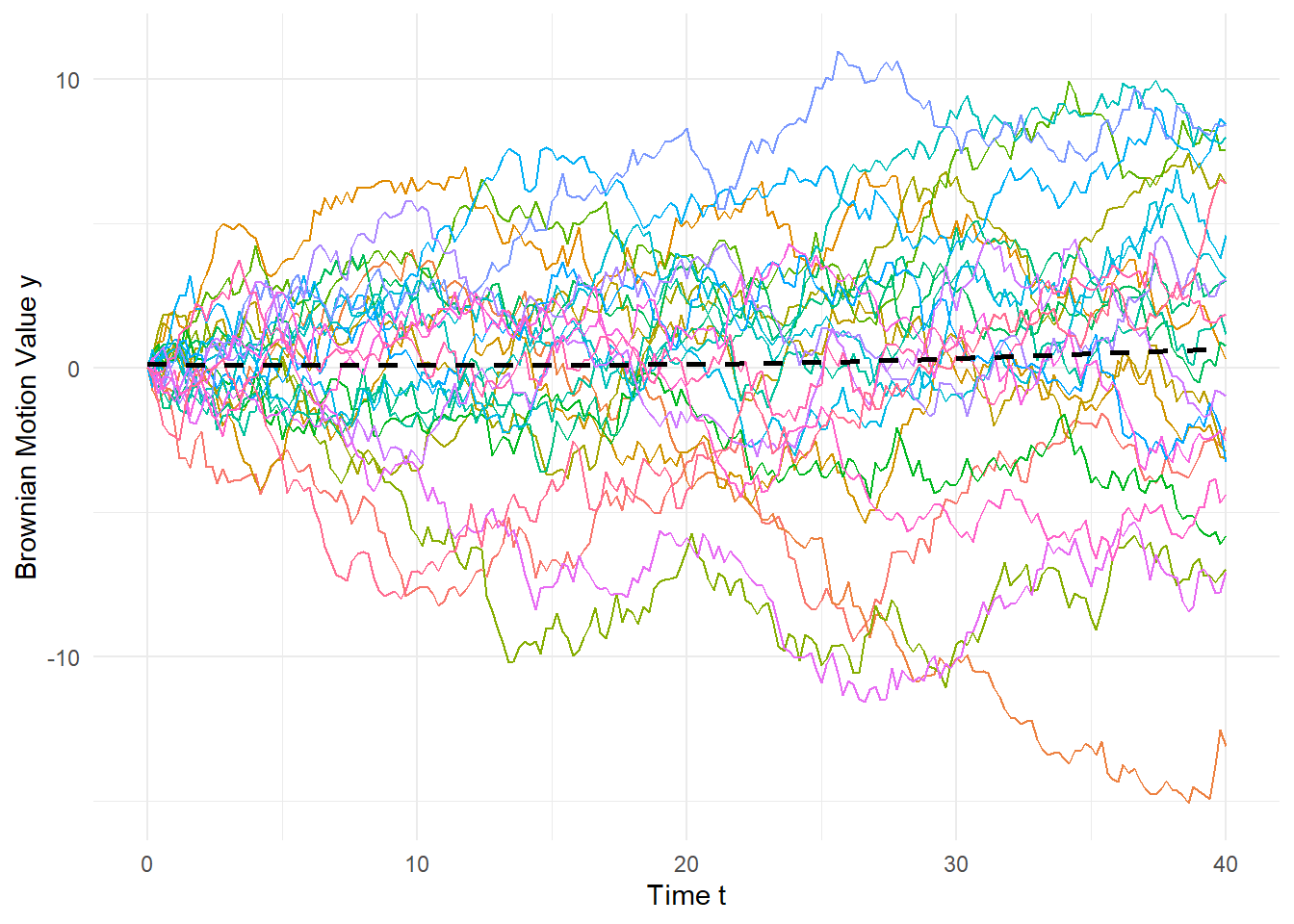
brownian_motion(40, 25, .2) %>%
  ggplot(aes(x = t, y = y, group = sim_number, color = sim_number)) +
  geom_line() +
  geom_smooth(se = FALSE, 
              aes(group = FALSE), 
              color = "black", 
              linetype = "dashed") +
  theme_minimal() +
  labs(
    x = "Time t",
    y = "Brownian Motion Value y"
  ) +
  theme(legend.position = "none")

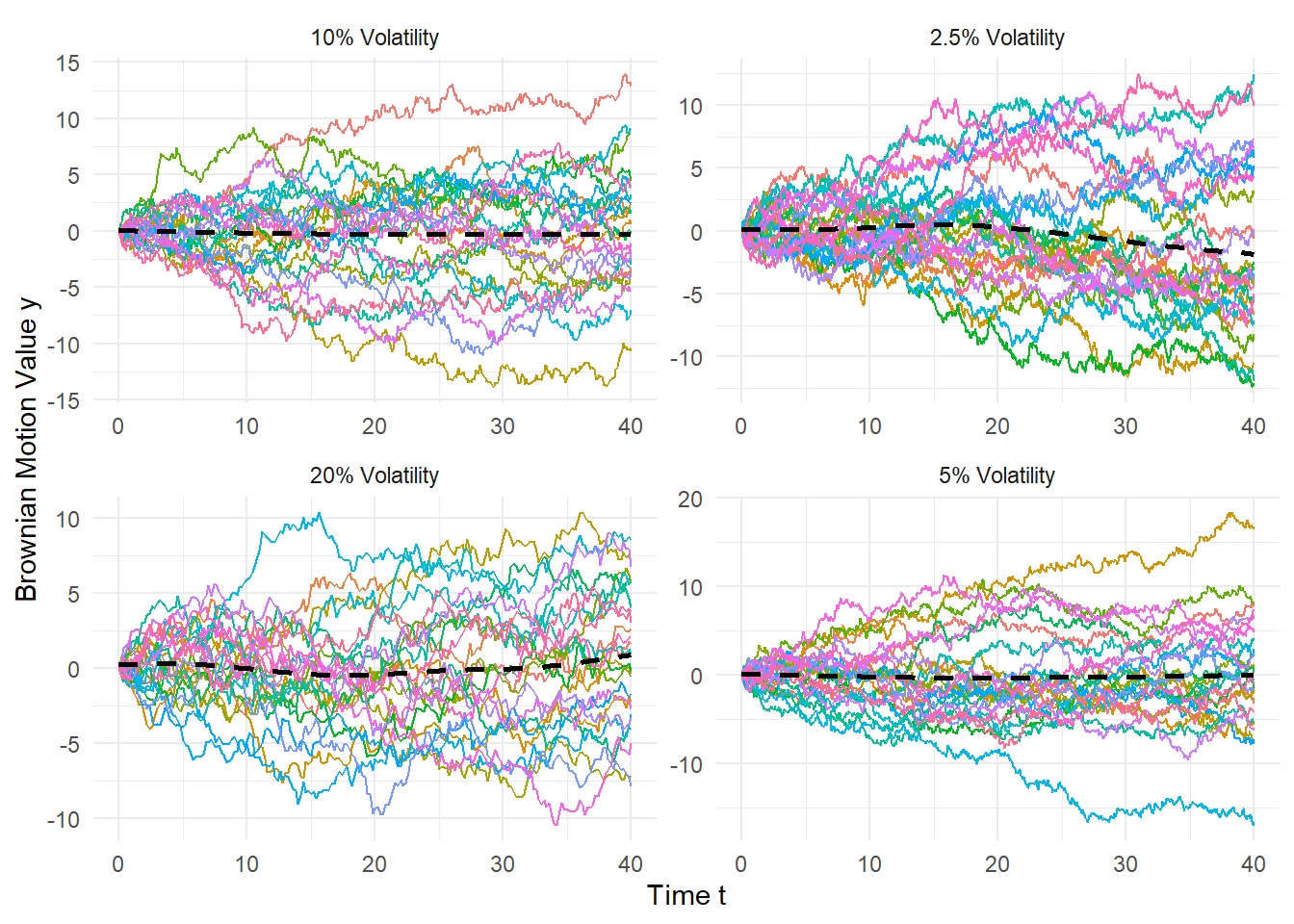
Now lets take a look at the change in a few different ones at the same time.

bm_tbl <- rbind(
  brownian_motion(40, 25, .2) %>%
    mutate(label = "20% Volatility"),
  brownian_motion(40, 25, .1) %>%
    mutate(label = "10% Volatility"),
  brownian_motion(40, 25, .05) %>%
    mutate(label = "5% Volatility"),
  brownian_motion(40, 25, .025) %>%
    mutate(label = "2.5% Volatility")
)

ggplot(bm_tbl, aes(x = t, y = y, group = sim_number, color = sim_number)) +
  geom_line() +
  facet_wrap(~ label, scales = "free") +
    geom_smooth(se = FALSE, 
              aes(group = FALSE), 
              color = "black", 
              linetype = "dashed") +
  theme_minimal() +
    labs(
    x = "Time t",
    y = "Brownian Motion Value y"
  ) +
  theme(legend.position = "none")

Voila!