Introduction

In time series analysis there is something called a lag. This simply means we take a look at some past event from some point in time t. This is a non-statistical method for looking at a relationship between a timeseries and its lags.

{healthyR.ts} has a function called ts_lag_correlation(). This function, as described by it’s name, provides more than just a simple lag plot.

This function provides a lot of extra information for the end user. First let’s go over the function call.

Function

Function Call

Here is the full call:

ts_lag_correlation(
  .data,
  .date_col,
  .value_col,
  .lags = 1,
  .heatmap_color_low = "white",
  .heatmap_color_hi = "steelblue"
)

Here are the arguments that get supplied to the different parameters.

.data - A tibble of time series data
.date_col - A date column
.value_col - The value column being analyzed
.lags - This is a vector of integer lags, ie 1 or c(1,6,12)
.heatmap_color_low - What color should the low values of the heatmap of the correlation matrix be, the default is ‘white’
.heatmap_color_hi - What color should the low values of the heatmap of the correlation matrix be, the default is ‘steelblue’

Function Return

The function itself returns a list object. The list has the following elements in it:

Data Elements

lag_list
lag_tbl
correlation_lag_matrix
correlation_lag_tbl

Plot Elements

lag_plot
plotly_lag_plot
correlation_heatmap
plotly_heatmap

Example

Let’s take a look at an example. We are going to use the built in data set of AirPassengers.

library(healthyR.ts)
library(dplyr)

df <- ts_to_tbl(AirPassengers) %>% select(-index)
lags <- c(1,3,6,12)

output <- ts_lag_correlation(
  .data = df,
  .date_col = date_col,
  .value_col = value,
  .lags = lags
)

Now that we have our output, let’s examine each piece of it.

Data Elements

Here are the data elements.

output$data$lag_list

[[1]]
# A tibble: 143 × 3
   lag   value lagged_value
   <fct> <dbl>        <dbl>
 1 1       118          112
 2 1       132          118
 3 1       129          132
 4 1       121          129
 5 1       135          121
 6 1       148          135
 7 1       148          148
 8 1       136          148
 9 1       119          136
10 1       104          119
# … with 133 more rows

[[2]]
# A tibble: 141 × 3
   lag   value lagged_value
   <fct> <dbl>        <dbl>
 1 3       129          112
 2 3       121          118
 3 3       135          132
 4 3       148          129
 5 3       148          121
 6 3       136          135
 7 3       119          148
 8 3       104          148
 9 3       118          136
10 3       115          119
# … with 131 more rows

[[3]]
# A tibble: 138 × 3
   lag   value lagged_value
   <fct> <dbl>        <dbl>
 1 6       148          112
 2 6       148          118
 3 6       136          132
 4 6       119          129
 5 6       104          121
 6 6       118          135
 7 6       115          148
 8 6       126          148
 9 6       141          136
10 6       135          119
# … with 128 more rows

[[4]]
# A tibble: 132 × 3
   lag   value lagged_value
   <fct> <dbl>        <dbl>
 1 12      115          112
 2 12      126          118
 3 12      141          132
 4 12      135          129
 5 12      125          121
 6 12      149          135
 7 12      170          148
 8 12      170          148
 9 12      158          136
10 12      133          119
# … with 122 more rows

This is a list of all the tibbles of the different lags that were chosen.

output$data$lag_tbl

# A tibble: 554 × 4
   lag   value lagged_value lag_title
   <fct> <dbl>        <dbl> <fct>    
 1 1       118          112 Lag: 1   
 2 1       132          118 Lag: 1   
 3 1       129          132 Lag: 1   
 4 1       121          129 Lag: 1   
 5 1       135          121 Lag: 1   
 6 1       148          135 Lag: 1   
 7 1       148          148 Lag: 1   
 8 1       136          148 Lag: 1   
 9 1       119          136 Lag: 1   
10 1       104          119 Lag: 1   
# … with 544 more rows

This is the long lag tibble with all of the lags in it.

output$data$correlation_lag_matrix

                value value_lag1 value_lag3 value_lag6 value_lag12
value       1.0000000  0.9542938  0.8186636  0.7657001   0.9905274
value_lag1  0.9542938  1.0000000  0.8828054  0.7726530   0.9492382
value_lag3  0.8186636  0.8828054  1.0000000  0.8349550   0.8218493
value_lag6  0.7657001  0.7726530  0.8349550  1.0000000   0.7780911
value_lag12 0.9905274  0.9492382  0.8218493  0.7780911   1.0000000

This is the correlation matrix.

output$data$correlation_lag_tbl

# A tibble: 25 × 3
   name        data_names value
   <fct>       <fct>      <dbl>
 1 value       value      1    
 2 value_lag1  value      0.954
 3 value_lag3  value      0.819
 4 value_lag6  value      0.766
 5 value_lag12 value      0.991
 6 value       value_lag1 0.954
 7 value_lag1  value_lag1 1    
 8 value_lag3  value_lag1 0.883
 9 value_lag6  value_lag1 0.773
10 value_lag12 value_lag1 0.949
# … with 15 more rows

This is the correlation lag tibble

Plot Elements

output$plots$lag_plot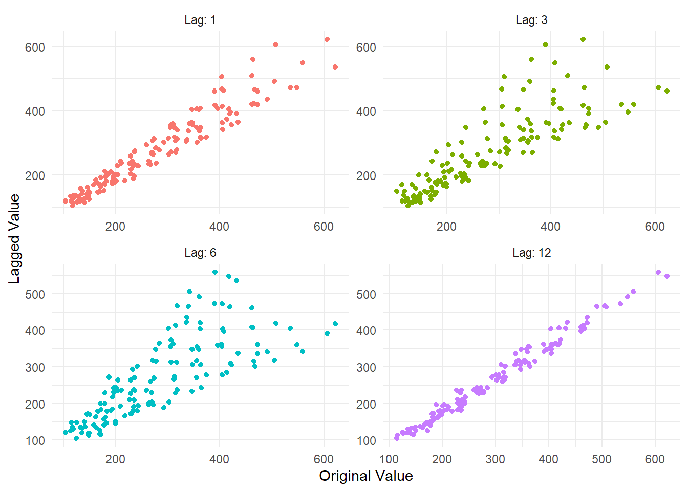

The Lag Plot itself.

output$plots$plotly_lag_plot

A plotly version of the lag plot.

output$plots$correlation_heatmap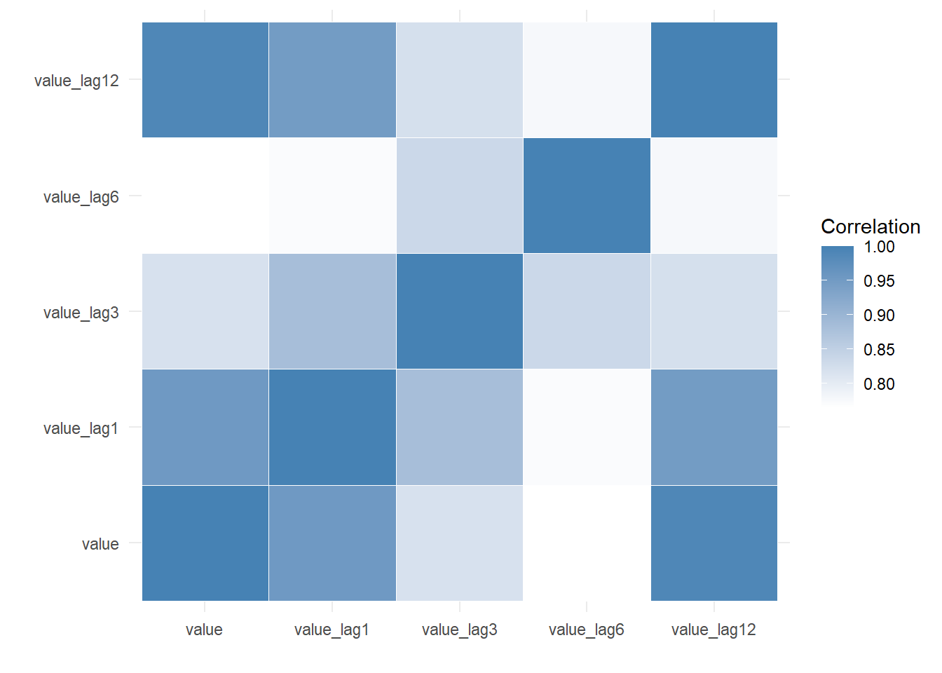

A heatmap of the correlations.

output$plots$plotly_heatmap

A plotly version of the correlation heatmap.

Voila!