Automatic Random Walks • RandomWalker

The simplest way to generate random walks with RandomWalker is using the automatic function rw30().

Overview

RandomWalker provides rw30() as a quick way to generate random walks without specifying any parameters. This is perfect for:

Quick demonstrations
Learning and teaching
Prototyping
Exploratory analysis

The rw30() Function

Basic Usage

# Generate 30 random walks
walks <- rw30()

# View the data
head(walks, 10)
#> # A tibble: 10 × 3
#>    walk_number step_number     y
#>    <fct>             <int> <dbl>
#>  1 1                     1  0   
#>  2 1                     2 -1.40
#>  3 1                     3 -1.14
#>  4 1                     4 -3.58
#>  5 1                     5 -3.59
#>  6 1                     6 -2.97
#>  7 1                     7 -1.82
#>  8 1                     8 -3.64
#>  9 1                     9 -3.89
#> 10 1                    10 -4.13

What rw30() Does

The rw30() function: 1. Generates 30 random walks 2. Each with 100 steps 3. Using normal distribution (mean = 0, sd = 1) 4. Starting at 0 5. Returns a tidy tibble

It’s equivalent to:

random_normal_walk(
  .num_walks = 30,
  .n = 100,
  .mu = 0,
  .sd = 1,
  .initial_value = 0,
  .dimensions = 1
)

Output Structure

rw30()
#> # A tibble: 3,000 × 3
#>    walk_number step_number     y
#>    <fct>             <int> <dbl>
#>  1 1                     1  0   
#>  2 1                     2  2.08
#>  3 1                     3  4.00
#>  4 1                     4  4.07
#>  5 1                     5  4.34
#>  6 1                     6  4.78
#>  7 1                     7  5.99
#>  8 1                     8  4.73
#>  9 1                     9  6.50
#> 10 1                    10  6.34
#> # ℹ 2,990 more rows

Columns: - walk_number: Factor (1-30) identifying each walk - step_number: Integer (1-100) for each step - y: The random walk values

Note: Cumulative columns such as cum_sum, cum_prod, cum_min, cum_max, and cum_mean are not included by default. You can add them using rand_walk_helper() or tidyverse operations if needed. ## Understanding the Output

Walk Structure

Each walk consists of 100 steps:

walks <- rw30()

# Count steps per walk
walks |>
  group_by(walk_number) |>
  summarize(n_steps = n()) |>
  head()
#> # A tibble: 6 × 2
#>   walk_number n_steps
#>   <fct>         <int>
#> 1 1               100
#> 2 2               100
#> 3 3               100
#> 4 4               100
#> 5 5               100
#> 6 6               100

Random Walk Behavior

Since steps are drawn from N(0,1):

# Mean of steps should be ≈ 0
mean(walks$y)
#> [1] 0.466777

# Standard deviation
sd(walks$y)
#> [1] 6.151453

# Final positions vary widely
walks |>
  group_by(walk_number) |>
  slice_max(step_number) |>
  pull(y) |>
  range()
#> [1] -21.96226  23.86830

Attributes

The function stores metadata:

walks <- rw30()
atb <- attributes(walks)
atb[!names(atb) %in% c("row.names", "class")]
#> $names
#> [1] "walk_number" "step_number" "y"          
#> 
#> $num_walks
#> [1] 30
#> 
#> $num_steps
#> [1] 100
#> 
#> $mu
#> [1] 0
#> 
#> $sd
#> [1] 1
#> 
#> $fns
#> [1] "rw30"
#> 
#> $dimension
#> [1] 1

Common Usage Patterns

Pattern 1: Quick Visualization

# One line to plot
rw30() |> visualize_walks()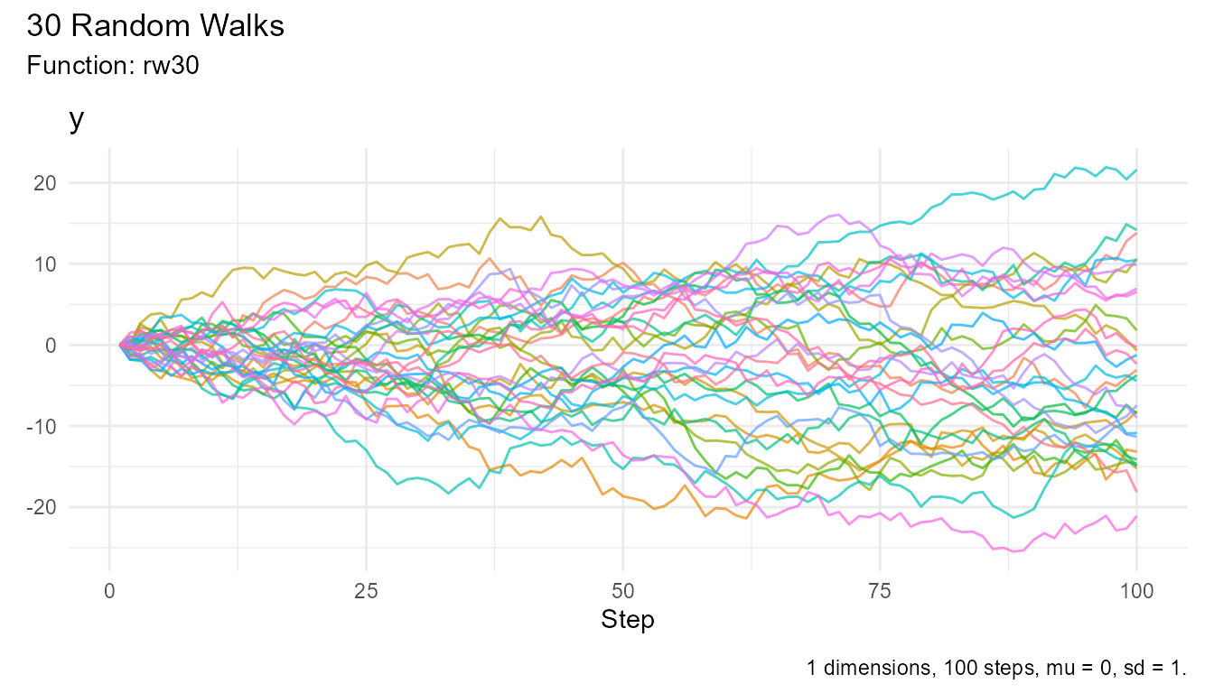

Line plot showing 30 random walks over 100 steps each. Each walk is represented by a different colored line starting at zero and fluctuating randomly over time. The x-axis shows step number and the y-axis shows the walk values.

# Interactive exploration
rw30() |> visualize_walks(.interactive = TRUE)

Pattern 2: Statistical Analysis

# Overall statistics
rw30() |> summarize_walks(.value = y) |>
  head()
#> Registered S3 method overwritten by 'quantmod':
#>   method            from
#>   as.zoo.data.frame zoo
#> Warning: There was 1 warning in `dplyr::summarize()`.
#> ℹ In argument: `geometric_mean = exp(mean(log(y)))`.
#> Caused by warning in `log()`:
#> ! NaNs produced
#> # A tibble: 1 × 16
#>   fns   fns_name dimensions mean_val median range quantile_lo quantile_hi
#>   <chr> <chr>         <dbl>    <dbl>  <dbl> <dbl>       <dbl>       <dbl>
#> 1 rw30  Rw30              1     1.42   1.22  49.3       -14.3        16.5
#> # ℹ 8 more variables: variance <dbl>, sd <dbl>, min_val <dbl>, max_val <dbl>,
#> #   harmonic_mean <dbl>, geometric_mean <dbl>, skewness <dbl>, kurtosis <dbl>

# By walk
rw30() |>
  summarize_walks(.value = y, .group_var = walk_number) |>
  head(10)
#> Warning: There were 28 warnings in `dplyr::summarize()`.
#> The first warning was:
#> ℹ In argument: `geometric_mean = exp(mean(log(y)))`.
#> ℹ In group 1: `walk_number = 1`.
#> Caused by warning in `log()`:
#> ! NaNs produced
#> ℹ Run `dplyr::last_dplyr_warnings()` to see the 27 remaining warnings.
#> # A tibble: 10 × 17
#>    walk_number fns   fns_name dimensions mean_val  median range quantile_lo
#>    <fct>       <chr> <chr>         <dbl>    <dbl>   <dbl> <dbl>       <dbl>
#>  1 1           rw30  Rw30              1  -11.6   -11.8    22.9     -21.8  
#>  2 2           rw30  Rw30              1    5.31    5.24   11.3       0.953
#>  3 3           rw30  Rw30              1   -6.67   -7.08   15.9     -13.8  
#>  4 4           rw30  Rw30              1   11.2    11.6    18.1       2.54 
#>  5 5           rw30  Rw30              1    1.14    1.06   10.2      -2.39 
#>  6 6           rw30  Rw30              1   -4.35   -4.32   13.8     -11.7  
#>  7 7           rw30  Rw30              1    8.56    8.86   20.6      -0.796
#>  8 8           rw30  Rw30              1    5.96    6.54   14.1      -2.20 
#>  9 9           rw30  Rw30              1   -1.42   -1.42   10.0      -5.75 
#> 10 10          rw30  Rw30              1   -0.835  -0.704  10.2      -4.81 
#> # ℹ 9 more variables: quantile_hi <dbl>, variance <dbl>, sd <dbl>,
#> #   min_val <dbl>, max_val <dbl>, harmonic_mean <dbl>, geometric_mean <dbl>,
#> #   skewness <dbl>, kurtosis <dbl>

# Custom analysis
rw30() |>
  group_by(walk_number) |>
  summarize(
    final_value = last(y),
    max_value = max(y),
    min_value = min(y),
    volatility = sd(y)
  ) |>
  head(10)
#> # A tibble: 10 × 5
#>    walk_number final_value max_value min_value volatility
#>    <fct>             <dbl>     <dbl>     <dbl>      <dbl>
#>  1 1                 2.82      2.95      -8.95       2.92
#>  2 2               -27.0       1.14     -27.0        7.77
#>  3 3                -8.33      1.85     -11.2        2.86
#>  4 4               -10.4       0.938    -13.3        3.24
#>  5 5                10.8      12.3       -2.20       3.67
#>  6 6                -6.39      3.53     -16.9        5.62
#>  7 7                 0.240     4.65      -7.20       2.84
#>  8 8               -12.0       0.553    -12.3        3.24
#>  9 9                 6.88     10.2       -6.06       4.37
#> 10 10               11.7      17.5       -3.05       5.22

Pattern 3: Finding Extremes

# Walk that went highest
max_walk <- rw30() |>
  subset_walks(.value = "y", .type = "max")

# Walk that went lowest
min_walk <- rw30() |>
  subset_walks(.value = "y", .type = "min")

# Visualize extremes
max_walk |> visualize_walks()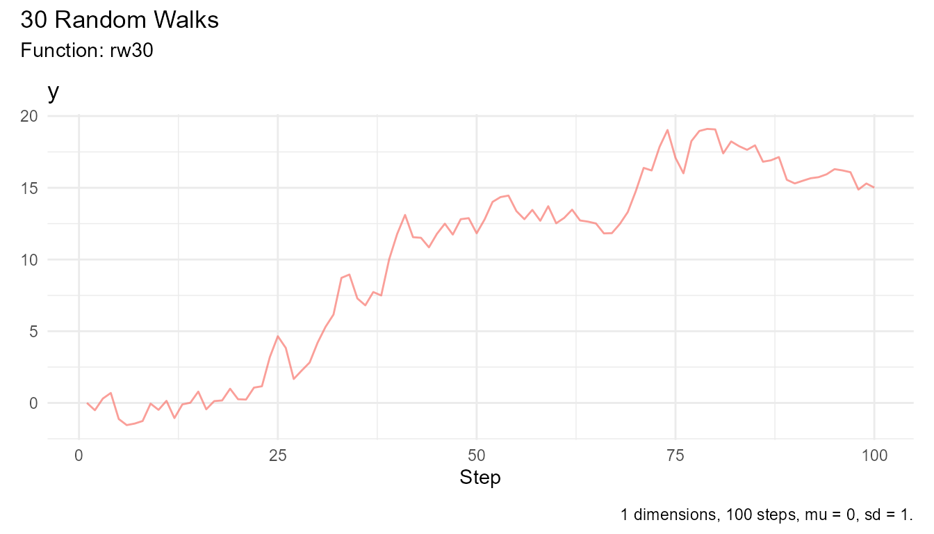

Line plot showing a single random walk that reached the highest maximum value among 30 walks. The line shows the walk's trajectory from start to finish, highlighting the extreme positive excursion.

Pattern 4: Filtering and Subsetting

walks <- rw30()

# Get only first 10 walks
walks |>
  filter(walk_number %in% as.character(1:10)) |>
  visualize_walks()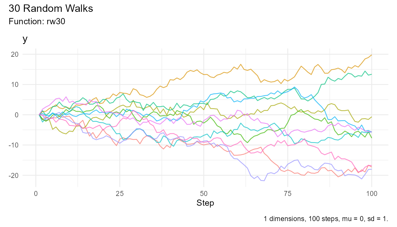

Line plot showing a subset of 10 random walks out of 30, filtered to display only walks numbered 1 through 10. Each walk is shown as a colored line progressing over 100 steps.

# Get steps 50-100 only
walks |>
  filter(step_number >= 50) |>
  visualize_walks()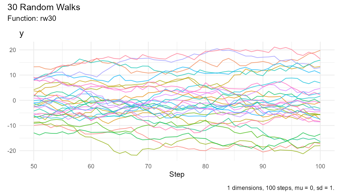

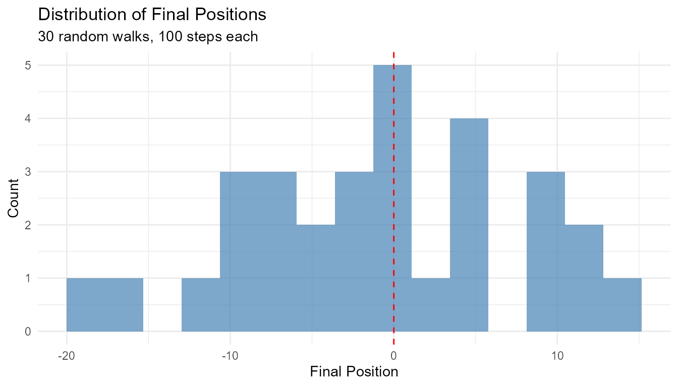
Line plot showing 30 random walks displaying only steps 50 through 100, showing the latter half of each walk's trajectory. The walks continue from their positions at step 50 rather than starting from zero.

Pattern 5: Teaching Demonstrations

# Show variability
walks <- rw30()

# Distribution of final positions
walks |>
  group_by(walk_number) |>
  slice_max(step_number) |>
  ggplot(aes(x = y)) +
  geom_histogram(bins = 15, fill = "steelblue", alpha = 0.7) +
  geom_vline(xintercept = 0, color = "red", linetype = "dashed") +
  theme_minimal() +
  labs(
    title = "Distribution of Final Positions",
    subtitle = "30 random walks, 100 steps each",
    x = "Final Position",
    y = "Count"
  )

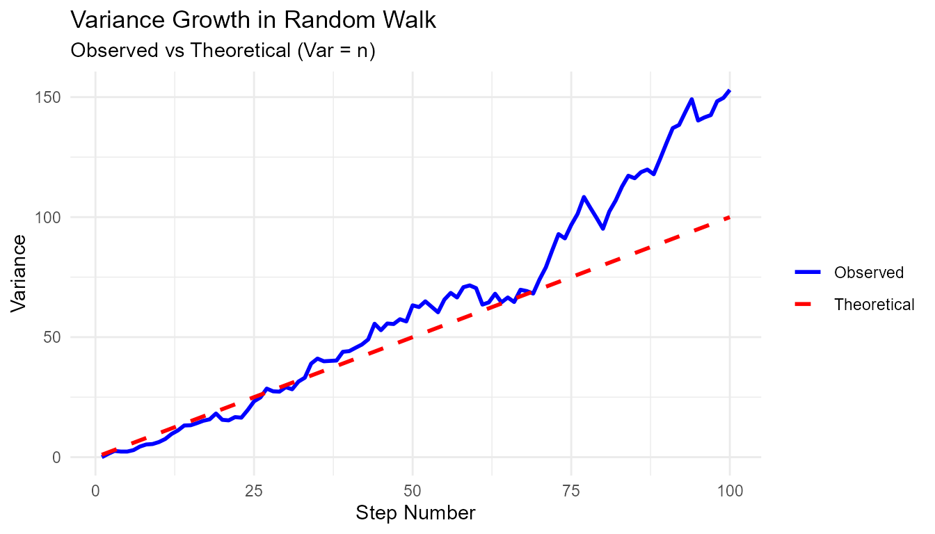
Histogram showing the distribution of final positions from 30 random walks after 100 steps. The distribution is centered around zero (marked by a red dashed vertical line) and shows a roughly bell-shaped spread of final values.

Pattern 6: Comparing to Theory

# Test if variance grows linearly with steps
walks <- rw30()

variance_by_step <- walks |>
  group_by(step_number) |>
  reframe(
    variance = var(y),
    theoretical = step_number  # For N(0,1), var = n
  )

ggplot(variance_by_step, aes(x = step_number)) +
  geom_line(aes(y = variance, color = "Observed"), linewidth = 1) +
  geom_line(aes(y = theoretical, color = "Theoretical"), linewidth = 1, linetype = "dashed") +
  scale_color_manual(values = c("Observed" = "blue", "Theoretical" = "red")) +
  theme_minimal() +
  labs(
    title = "Variance Growth in Random Walk",
    subtitle = "Observed vs Theoretical (Var = n)",
    x = "Step Number",
    y = "Variance",
    color = ""
  )

Line plot comparing observed variance (blue solid line) versus theoretical variance (red dashed line) as a function of step number. The observed variance closely tracks the theoretical prediction that variance equals the number of steps, demonstrating that variance grows linearly with the number of steps.

When to Use rw30()

✅ Use rw30() When:

Learning: First time using RandomWalker
Demos: Quick demonstrations
Teaching: Showing random walk concepts
Prototyping: Testing visualization or analysis code
Exploratory: Quick data exploration

❌ Don’t Use rw30() When:

Custom parameters needed: Use random_normal_walk() instead
Different distribution: Use specific generator functions
Different number of walks: rw30() always generates 30
Multi-dimensional: rw30() is 1D only
Production code: Use explicit generator functions for clarity

Limitations

Fixed Parameters

rw30() has no parameters, which means:

# ❌ Can't change number of walks
# rw30(.num_walks = 50)  # Error!

# ✅ Use random_normal_walk() instead
random_normal_walk(.num_walks = 50)

# ❌ Can't change number of steps
# rw30(.n = 200)  # Error!

# ✅ Use random_normal_walk() instead
random_normal_walk(.n = 200)

# ❌ Can't change distribution parameters
# rw30(.mu = 0.1)  # Error!

# ✅ Use random_normal_walk() instead
random_normal_walk(.mu = 0.1)

Only Normal Distribution

rw30() uses normal distribution exclusively:

# ❌ Can't use other distributions
# rw30(.distribution = "cauchy")  # Not possible!

# ✅ Use specific generator functions
random_cauchy_walk(.num_walks = 30)
geometric_brownian_motion(.num_walks = 30)
discrete_walk(.num_walks = 30)

Only 1D

rw30() generates 1D walks only:

# ❌ Can't create 2D walks
# rw30(.dimensions = 2)  # Error!

# ✅ Use random_normal_walk()
random_normal_walk(.num_walks = 30, .dimensions = 2)

Alternatives to rw30()

When rw30() doesn’t fit your needs:

For Custom Parameters

# Instead of rw30()
random_normal_walk(
  .num_walks = 30,
  .n = 100,
  .mu = 0,
  .sd = 1,
  .initial_value = 0
)

# With custom parameters
random_normal_walk(
  .num_walks = 50,
  .n = 200,
  .mu = 0.05,
  .sd = 0.5,
  .initial_value = 100
)

For Different Distributions

# Geometric Brownian Motion (like rw30 but for stocks)
geometric_brownian_motion(
  .num_walks = 30,
  .n = 100,
  .initial_value = 100
)

# Heavy-tailed walks
random_cauchy_walk(
  .num_walks = 30,
  .n = 100
)

# Discrete walks
discrete_walk(
  .num_walks = 30,
  .n = 100
)

For Multi-Dimensional

# 2D walks
random_normal_walk(
  .num_walks = 30,
  .n = 100,
  .dimensions = 2
)

# 3D walks
random_normal_walk(
  .num_walks = 30,
  .n = 100,
  .dimensions = 3
)

Complete Examples

Example 1: Teaching Random Walk Properties

# Generate walks
walks <- rw30()

# Show that mean displacement is zero
walks |>
  group_by(step_number) |>
  summarize(mean_position = mean(y)) |>
  ggplot(aes(x = step_number, y = mean_position)) +
  geom_line(color = "blue", linewidth = 1) +
  geom_hline(yintercept = 0, linetype = "dashed", color = "red") +
  theme_minimal() +
  labs(
    title = "Mean Position Over Time",
    subtitle = "Averages to zero (red line)",
    x = "Step",
    y = "Mean Position"
  )

Line plot showing the mean position across all 30 walks as a function of step number. The mean fluctuates around zero (marked by a red dashed horizontal line), demonstrating that random walks have zero expected displacement.

# Show that standard deviation grows as sqrt(n)
walks |>
  group_by(step_number) |>
  reframe(
    sd_position = sd(y),
    theoretical = sqrt(step_number)
  ) |>
  ungroup() |>
  ggplot(aes(x = step_number)) +
  geom_line(aes(y = sd_position, color = "Observed"), linewidth = 1) +
  geom_line(aes(y = theoretical, color = "Theoretical"), linewidth = 1, linetype = "dashed") +
  scale_color_manual(values = c("Observed" = "blue", "Theoretical" = "red")) +
  theme_minimal() +
  labs(
    title = "Standard Deviation Growth",
    subtitle = "Should follow sqrt(n) (red dashed line)",
    x = "Step",
    y = "Standard Deviation",
    color = ""
  )

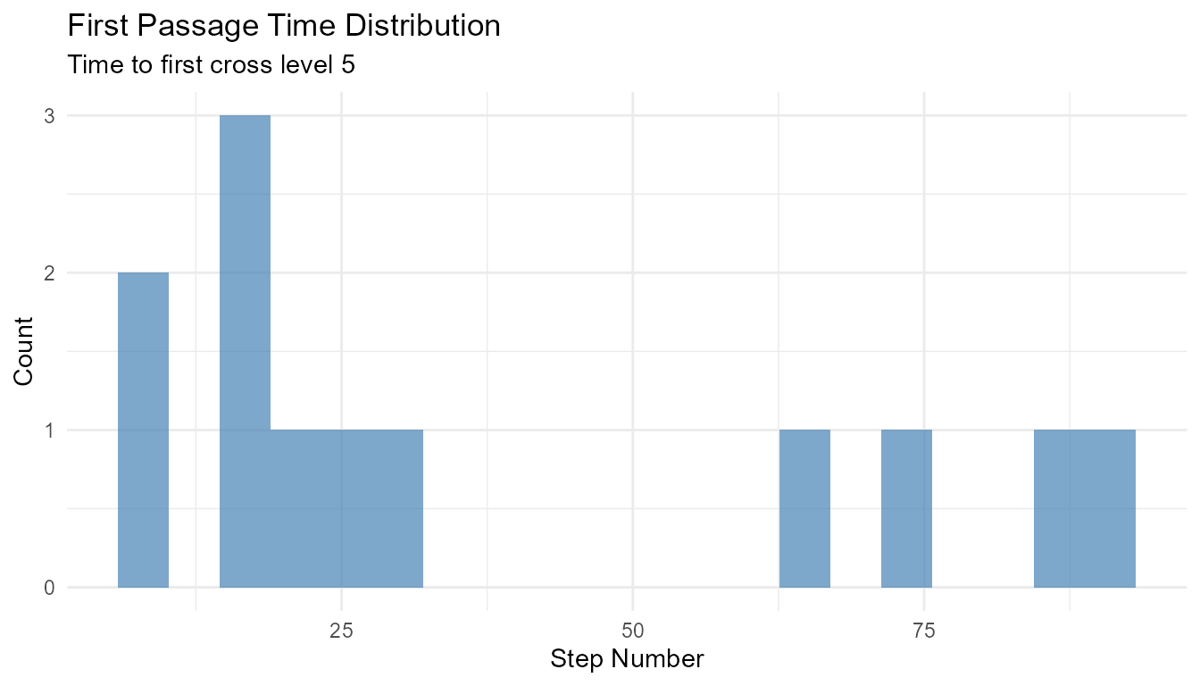
Line plot comparing observed standard deviation (blue solid line) versus theoretical standard deviation (red dashed line) as a function of step number. The observed standard deviation closely follows the theoretical sqrt(n) relationship, demonstrating that random walk spread grows as the square root of time.

Example 2: First Passage Time

# Find when walks first cross a threshold
walks <- rw30()

first_crossing <- walks |>
  group_by(walk_number) |>
  filter(y >= 5) |>
  slice_min(step_number, n = 1) |>
  select(walk_number, first_crossing_time = step_number)

# Some walks may never cross
n_crossed <- nrow(first_crossing)
cat(sprintf("%d out of 30 walks crossed 5\n", n_crossed))
#> 12 out of 30 walks crossed 5

# Distribution of first crossing times
if (n_crossed > 0) {
  ggplot(first_crossing, aes(x = first_crossing_time)) +
    geom_histogram(bins = 20, fill = "steelblue", alpha = 0.7) +
    theme_minimal() +
    labs(
      title = "First Passage Time Distribution",
      subtitle = "Time to first cross level 5",
      x = "Step Number",
      y = "Count"
    )
}

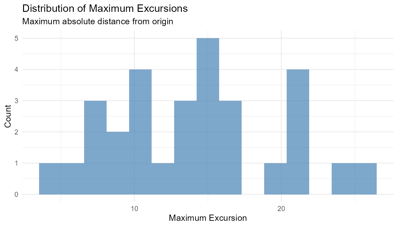
Histogram showing the distribution of first passage times - the step number at which walks first crossed the threshold value of 5. Only walks that successfully crossed the threshold are included, showing when they first exceeded the boundary.

Example 3: Maximum Excursion

# Find maximum distance from origin
walks <- rw30()

max_excursion <- walks |>
  group_by(walk_number) |>
  summarize(
    max_positive = max(y),
    max_negative = min(y),
    max_excursion = max(abs(y))
  )

# Visualize
max_excursion |>
  ggplot(aes(x = max_excursion)) +
  geom_histogram(bins = 15, fill = "steelblue", alpha = 0.7) +
  theme_minimal() +
  labs(
    title = "Distribution of Maximum Excursions",
    subtitle = "Maximum absolute distance from origin",
    x = "Maximum Excursion",
    y = "Count"
  )

Histogram showing the distribution of maximum excursions - the largest absolute distance each walk reached from the origin during its 100 steps. The distribution shows how far walks typically strayed from their starting point.

Next Steps

Once you’re comfortable with rw30(), explore:

Getting Started Guide - Learn more random walk functions with vignette("getting-started")
Function Reference - Explore all distributions at the package website
Home Wiki - Learn about visualization and statistical analysis with vignette("home")

Ready for more control? Check out the function reference for customizable random walks!