Basic Concepts

Understanding the fundamentals of random walks and how RandomWalker implements them.

What is a Random Walk?
Types of Random Walks
Key Properties
Mathematical Background
RandomWalker Implementation
Common Terminology

What is a Random Walk?

A random walk is a mathematical model describing a path consisting of a succession of random steps. At each point in time, the next step is determined by chance.

Simple Example

Imagine flipping a coin: - Heads: Move one step forward (+1) - Tails: Move one step backward (-1) - Start: Position 0

After 10 flips, you might be at position +2, -4, or anywhere else. This is a random walk!

# Coin flip random walk
coin_walk <- discrete_walk(
  .num_walks = 1,
  .n = 100,
  .upper_bound = 1,
  .lower_bound = -1,
  .upper_probability = 0.5
)

coin_walk |> visualize_walks(.pluck = "cum_sum")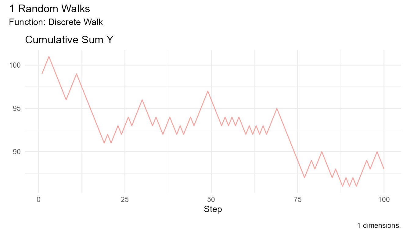

Line plot showing a single random walk simulating coin flips over 100 steps. The walk moves up or down by 1 with equal probability at each step, starting from position 0. The x-axis shows the step number and the y-axis shows the cumulative sum position.

Real-World Analogies

Stock prices: Daily price changes are like random steps
Particle motion: Molecules moving due to thermal energy
Drunk person walking: Each step in a random direction
Photon path: Light scattering through a medium

Types of Random Walks

1. Simple Random Walk

Each step is ±1 with equal probability:

discrete_walk(
  .num_walks = 10,
  .upper_bound = 1,
  .lower_bound = -1,
  .upper_probability = 0.5
) |> head(10)
#> # A tibble: 10 × 8
#>    walk_number step_number     y cum_sum_y cum_prod_y cum_min_y cum_max_y
#>    <fct>             <int> <dbl>     <dbl>      <dbl>     <dbl>     <dbl>
#>  1 1                     1     1       101        200       101       101
#>  2 1                     2     1       102        400       101       101
#>  3 1                     3    -1       101          0        99       101
#>  4 1                     4    -1       100          0        99       101
#>  5 1                     5    -1        99          0        99       101
#>  6 1                     6     1       100          0        99       101
#>  7 1                     7     1       101          0        99       101
#>  8 1                     8     1       102          0        99       101
#>  9 1                     9     1       103          0        99       101
#> 10 1                    10     1       104          0        99       101
#> # ℹ 1 more variable: cum_mean_y <dbl>

Properties: - Symmetric (unbiased) - Steps are independent - Mean position = 0 - Variance grows linearly with time

2. Random Walk with Drift

Steps have a non-zero mean (bias in one direction):

random_normal_drift_walk(
  .num_walks = 10,
  .drift = 0.1  # Positive drift
) |> head(10)
#> # A tibble: 10 × 8
#>    walk_number step_number       y cum_sum_y cum_prod_y cum_min_y cum_max_y
#>    <fct>             <int>   <dbl>     <dbl>      <dbl>     <dbl>     <dbl>
#>  1 1                     1 -1.47      -1.47           0     -1.47     -1.47
#>  2 1                     2 -2.49      -3.96           0     -2.49     -1.47
#>  3 1                     3  2.15      -1.81           0     -2.49      2.15
#>  4 1                     4  1.15      -0.654          0     -2.49      2.15
#>  5 1                     5  1.42       0.769          0     -2.49      2.15
#>  6 1                     6 -0.348      0.421          0     -2.49      2.15
#>  7 1                     7  0.769      1.19           0     -2.49      2.15
#>  8 1                     8  0.0966     1.29           0     -2.49      2.15
#>  9 1                     9  3.81       5.10           0     -2.49      3.81
#> 10 1                    10  0.984      6.09           0     -2.49      3.81
#> # ℹ 1 more variable: cum_mean_y <dbl>

Properties: - Asymmetric (biased) - Tends to move in one direction - Mean position ≠ 0 - Can model trending data

3. Brownian Motion (Wiener Process)

Continuous-time random walk:

brownian_motion(
  .num_walks = 10,
  .delta_time = 1
) |> head(10)
#> # A tibble: 10 × 8
#>    walk_number step_number        y cum_sum_y cum_prod_y cum_min_y cum_max_y
#>    <fct>             <int>    <dbl>     <dbl>      <dbl>     <dbl>     <dbl>
#>  1 1                     1  0.00165   0.00165          0   0.00165   0.00165
#>  2 1                     2 -1.19     -1.19             0  -1.19      0.00165
#>  3 1                     3  0.362    -0.823            0  -1.19      0.362  
#>  4 1                     4 -0.549    -1.37             0  -1.19      0.362  
#>  5 1                     5  0.693    -0.680            0  -1.19      0.693  
#>  6 1                     6 -0.0608   -0.741            0  -1.19      0.693  
#>  7 1                     7 -1.19     -1.93             0  -1.19      0.693  
#>  8 1                     8 -0.120    -2.05             0  -1.19      0.693  
#>  9 1                     9 -0.708    -2.76             0  -1.19      0.693  
#> 10 1                    10 -1.62     -4.38             0  -1.62      0.693  
#> # ℹ 1 more variable: cum_mean_y <dbl>

Properties: - Continuous in time - Normally distributed increments - Foundation of stochastic calculus - Used in physics and finance

4. Geometric Brownian Motion

Multiplicative random walk (always positive):

geometric_brownian_motion(
  .num_walks = 10,
  .initial_value = 100
) |> head(10)
#> # A tibble: 10 × 8
#>    walk_number step_number     y cum_sum_y cum_prod_y cum_min_y cum_max_y
#>    <fct>             <int> <dbl>     <dbl>      <dbl>     <dbl>     <dbl>
#>  1 1                     1  1.00      101.       200.      101.      101.
#>  2 1                     2  1.01      102.       403.      101.      101.
#>  3 1                     3  1.00      103.       807.      101.      101.
#>  4 1                     4  1.00      104.      1616.      101.      101.
#>  5 1                     5  1.01      105.      3245.      101.      101.
#>  6 1                     6  1.01      106.      6519.      101.      101.
#>  7 1                     7  1.01      107.     13136.      101.      101.
#>  8 1                     8  1.02      108.     26474.      101.      101.
#>  9 1                     9  1.02      109.     53464.      101.      101.
#> 10 1                    10  1.02      110.    107797.      101.      101.
#> # ℹ 1 more variable: cum_mean_y <dbl>

Properties: - Cannot go negative - Used for stock prices - Log-normal distribution - Percentage changes are normal

Key Properties

Property 1: Mean Displacement

For a symmetric random walk starting at 0:

Expected value after n steps = 0

# Verify empirically
walks <- random_normal_walk(.num_walks = 1000, .n = 100)

walks |>
  summarize(overall_mean = mean(cum_sum_y))
#> # A tibble: 1 × 1
#>   overall_mean
#>          <dbl>
#> 1      -0.0648

Property 2: Variance Growth

For standard random walk:

Variance after n steps = n

# Verify empirically
walks <- random_normal_walk(.num_walks = 1000, .n = 100)

walks |>
  filter(step_number == 80) |>
  summarize(
    variance = var(cum_sum_y),
    theoretical = 80
  )
#> # A tibble: 1 × 2
#>   variance theoretical
#>      <dbl>       <dbl>
#> 1     1.45          80

Property 3: Distance from Origin

Expected distance grows as √n:

E[|position|] ∝ √n

# Verify with 2D walk
walks_2d <- random_normal_walk(.num_walks = 100, .n = 500, .dimensions = 2)

walks_2d |>
  euclidean_distance(.x = x, .y = y) |>
  group_by(step_number) |>
  reframe(
    mean_distance = mean(distance),
    theoretical = sqrt(step_number)
  ) |>
  filter(step_number %% 50 == 0) |>
  head(10)
#> # A tibble: 10 × 3
#>    step_number mean_distance theoretical
#>          <int>         <dbl>       <dbl>
#>  1          50         0.180        7.07
#>  2          50         0.180        7.07
#>  3          50         0.180        7.07
#>  4          50         0.180        7.07
#>  5          50         0.180        7.07
#>  6          50         0.180        7.07
#>  7          50         0.180        7.07
#>  8          50         0.180        7.07
#>  9          50         0.180        7.07
#> 10          50         0.180        7.07

Property 4: First Return to Origin

For 1D symmetric walk: - Probability of eventual return = 1 (certain to return) - Expected return time = ∞ (infinite expected time!)

For 2D symmetric walk: - Probability of eventual return = 1

For 3D symmetric walk: - Probability of eventual return ≈ 0.34 (not certain!)

Property 5: Scaling

Random walks exhibit scaling invariance: - If you zoom out by factor k - Time scales by k² - Position scales by k

Mathematical Background

One-Dimensional Random Walk

Position after n steps:

X(n) = X(0) + Σ(i=1 to n) Δᵢ

Where Δᵢ are independent random steps.

For standard normal walk: - Δᵢ ~ N(0, 1) - X(n) ~ N(0, n) - E[X(n)] = 0 - Var[X(n)] = n

Brownian Motion

Continuous-time stochastic process:

dX(t) = μ dt + σ dW(t)

Where: - μ = drift coefficient - σ = volatility coefficient - W(t) = standard Wiener process

Properties: - W(0) = 0 - W(t) ~ N(0, t) - W(t) - W(s) ~ N(0, t-s) for t > s - Independent increments

Geometric Brownian Motion

For stock prices:

dS(t) = μ S(t) dt + σ S(t) dW(t)

Solution:

S(t) = S(0) exp((μ - σ²/2)t + σW(t))

Properties: - Always positive - Log-normal distribution - Used in Black-Scholes model

RandomWalker Implementation

How RandomWalker Works

Generate random steps from specified distribution
Compute cumulative sum (position over time)
Add cumulative statistics (min, max, mean, product)
Return tidy tibble for analysis

Example: Behind the Scenes

# What rw30() does internally:

# 1. Generate random steps
steps <- rnorm(100, mean = 0, sd = 1)

# 2. Compute cumulative sum
positions <- cumsum(c(0, steps[-100]))

# 3. Add to tibble
walk_data <- tibble::tibble(
  step_number = 1:100,
  y = steps,
  cum_sum = positions
)

# 4. Add more cumulative functions
walk_data <- walk_data |>
  mutate(
    cum_prod = cumprod(1 + y),
    cum_min = cummin(y),
    cum_max = cummax(y),
    cum_mean = cumsum(y) / step_number
  )

walk_data |> head(10)
#> # A tibble: 10 × 7
#>    step_number      y cum_sum cum_prod cum_min cum_max cum_mean
#>          <int>  <dbl>   <dbl>    <dbl>   <dbl>   <dbl>    <dbl>
#>  1           1 -1.18   0       -0.176    -1.18  -1.18  -1.18   
#>  2           2  0.607 -1.18    -0.282    -1.18   0.607 -0.284  
#>  3           3  0.552 -0.569   -0.438    -1.18   0.607 -0.00553
#>  4           4  0.455 -0.0166  -0.637    -1.18   0.607  0.110  
#>  5           5  0.181  0.438   -0.752    -1.18   0.607  0.124  
#>  6           6 -1.25   0.619    0.187    -1.25   0.607 -0.105  
#>  7           7  1.67  -0.630    0.499    -1.25   1.67   0.148  
#>  8           8 -0.761  1.04     0.120    -1.25   1.67   0.0346 
#>  9           9  1.14   0.277    0.256    -1.25   1.67   0.157  
#> 10          10 -0.644  1.42     0.0910   -1.25   1.67   0.0772

Dimensions

1D Walk: - Single value per step: y - Position: cum_sum

2D Walk: - Two values per step: x, y - Position: (cum_sum_x, cum_sum_y) - Distance: sqrt(cum_sum_x² + cum_sum_y²)

3D Walk: - Three values per step: x, y, z - Position: (cum_sum_x, cum_sum_y, cum_sum_z) - Distance: sqrt(cum_sum_x² + cum_sum_y² + cum_sum_z²)

Common Terminology

Terms Used in RandomWalker

Term	Definition	Example
Walk	A single realization of the random process	One stock price path
Step	One random increment	Daily price change
Trajectory	Path taken by the walk	Price history
Cumulative sum	Running total of steps	Stock price level
Displacement	Distance from starting point	Profit/loss
Excursion	Distance from reference point	Drawdown
First passage time	Time to first reach a level	Time to profit
Return time	Time to return to starting point	Recovery time

Statistical Terms

Term	Definition
Mean	Average value
Variance	Spread of values
Standard deviation	√Variance
Skewness	Asymmetry measure
Kurtosis	Tail heaviness
Quantile	Percentile value
Confidence interval	Range containing true value with probability

Probability Distributions

Distribution	Use Case	Parameters
Normal	General purpose	μ (mean), σ (sd)
Uniform	Equal probabilities	min, max
Exponential	Waiting times	λ (rate)
Poisson	Event counts	λ (rate)
Cauchy	Heavy tails	location, scale
Binomial	Success counts	n (trials), p (prob)

Worked Examples

Example 1: Verify Properties

# Generate many walks
walks <- random_normal_walk(.num_walks = 1000, .n = 100)

# Property 1: Mean = 0
walks |>
  summarize(overall_mean = mean(cum_sum_y))
#> # A tibble: 1 × 1
#>   overall_mean
#>          <dbl>
#> 1       0.0275

# Property 2: Variance = n
walks |>
  filter(step_number == 80) |>
  summarize(
    variance = var(cum_sum_y),
    theoretical = 80
  )
#> # A tibble: 1 × 2
#>   variance theoretical
#>      <dbl>       <dbl>
#> 1     1.39          80

# Property 3: Distance ∝ √n
walks |>
  group_by(step_number) |>
  summarize(
    mean_abs_position = mean(abs(cum_sum_y)),
    theoretical = sqrt(2/pi) * sqrt(step_number)  # Exact for normal
  ) |>
  filter(step_number %% 20 == 0) |>
  head(5)
#> Warning: Returning more (or less) than 1 row per `summarise()` group was deprecated in
#> dplyr 1.1.0.
#> ℹ Please use `reframe()` instead.
#> ℹ When switching from `summarise()` to `reframe()`, remember that `reframe()`
#>   always returns an ungrouped data frame and adjust accordingly.
#> Call `lifecycle::last_lifecycle_warnings()` to see where this warning was
#> generated.
#> `summarise()` has grouped output by 'step_number'. You can override using the
#> `.groups` argument.
#> # A tibble: 5 × 3
#> # Groups:   step_number [1]
#>   step_number mean_abs_position theoretical
#>         <int>             <dbl>       <dbl>
#> 1          20             0.390        3.57
#> 2          20             0.390        3.57
#> 3          20             0.390        3.57
#> 4          20             0.390        3.57
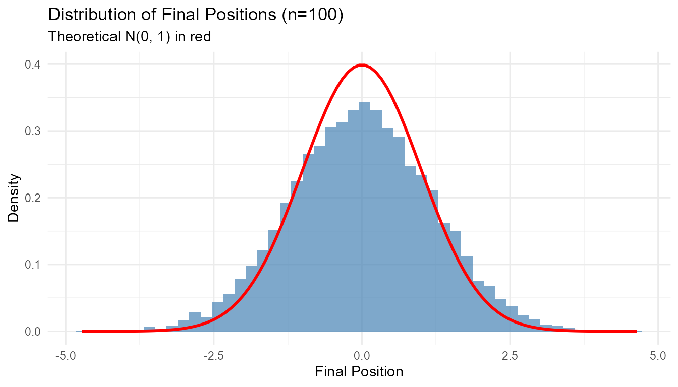
#> 5          20             0.390        3.57

Example 2: Distribution of Final Position

# Generate walks
walks <- random_normal_walk(.num_walks = 10000, .n = 100)

# Get final positions
final_pos <- walks |>
  group_by(walk_number) |>
  slice_max(step_number) |>
  pull(cum_sum_y)

# Plot
tibble::tibble(position = final_pos) |>
  ggplot(aes(x = position)) +
  geom_histogram(aes(y = after_stat(density)), bins = 50,
                 fill = "steelblue", alpha = 0.7) +
  stat_function(fun = dnorm, args = list(mean = 0, sd = 1),
                color = "red", linewidth = 1) +
  theme_minimal() +
  labs(
    title = "Distribution of Final Positions (n=100)",
    subtitle = "Theoretical N(0, 1) in red",
    x = "Final Position",
    y = "Density"
  )

Histogram showing the distribution of final positions for 10,000 random walks after 100 steps each. The histogram uses blue bars showing the empirical density, overlaid with a red curve representing the theoretical normal distribution N(0, 1). The distribution is centered near 0 with spread approximately 1, demonstrating that final positions follow a normal distribution.

Example 3: Path Dependency

Random walks are path-dependent - the ending doesn’t tell you the route:

# Generate walks ending at similar positions
set.seed(123)
walks <- random_normal_walk(.num_walks = 100, .n = 100)

# Find walks ending near 10
similar_end <- walks |>
  group_by(walk_number) |>
  filter(step_number == 80, abs(cum_sum_y - 1) < 0.5)

# Plot their paths - very different!
walks |>
  filter(walk_number %in% similar_end$walk_number) |>
  visualize_walks(.pluck = "cum_sum", .alpha = 0.5)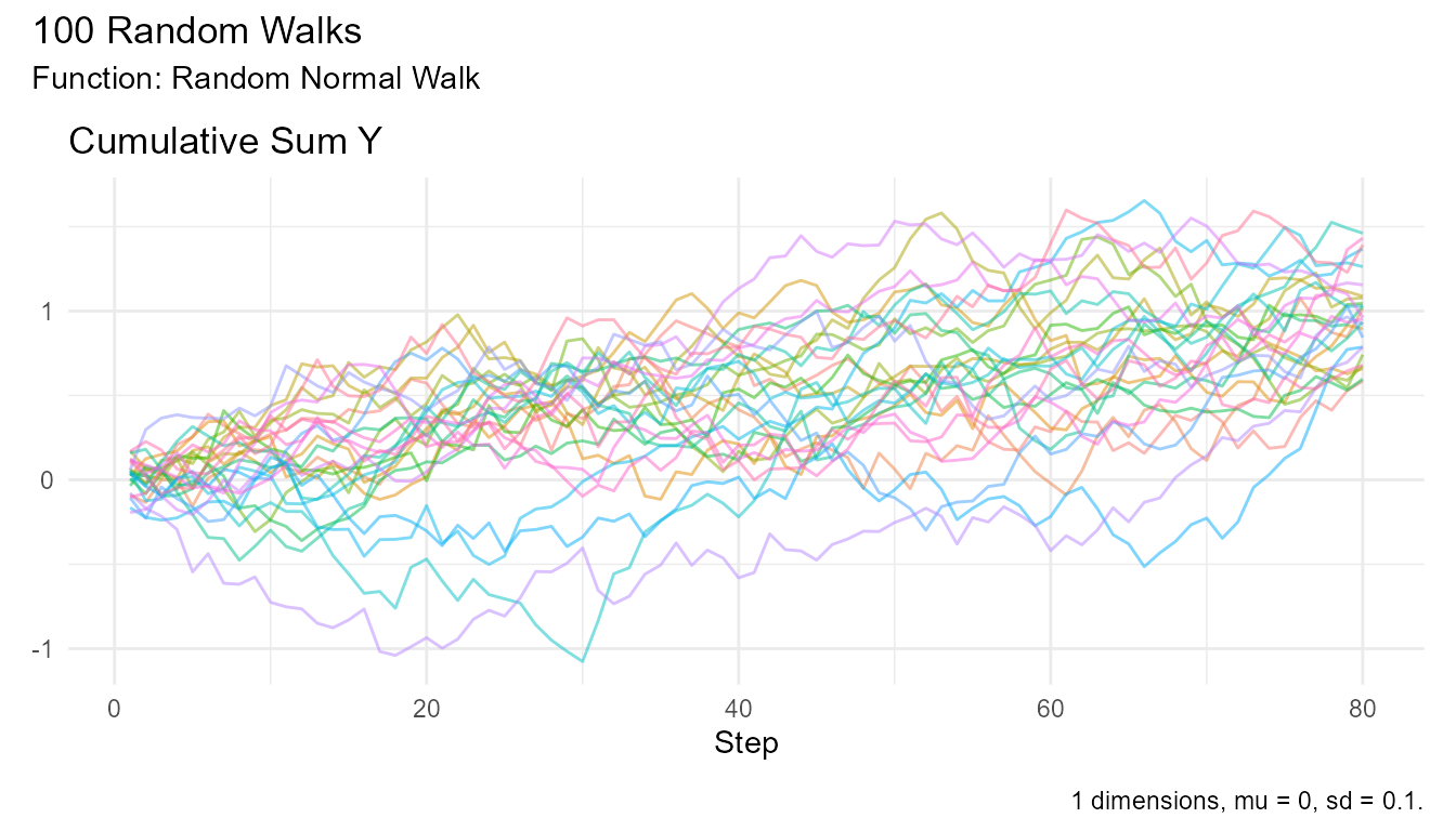

Line plot showing multiple random walk trajectories that pass through similar positions (near 1 at step 80) but take very different paths. Each semi-transparent line shows the complete 100-step trajectory of one walk, demonstrating path dependency - walks passing through the same point can have very different histories and futures.

Next Steps

Now that you understand the basics:

Quick Start Guide - Start using RandomWalker (see Getting Started vignette)
Continuous Distribution Generators - Explore distributions (see API Reference)
Statistical Analysis Guide - Analyze properties
Use Cases and Examples - Real-world applications

Table of Contents