Continuous Distribution Generators

RandomWalker provides a comprehensive suite of random walk generators based on continuous probability distributions. Each function follows a consistent API design for ease of use.

Common Parameters
Normal Distribution
Brownian Motion
Geometric Brownian Motion
Beta Distribution
Cauchy Distribution
Chi-Squared Distribution
Exponential Distribution
F Distribution
Gamma Distribution
Log-Normal Distribution
Logistic Distribution
Student’s t Distribution
Uniform Distribution
Weibull Distribution
Comparison Guide

Common Parameters

All continuous distribution generators share these common parameters:

Parameter	Type	Description	Default
`.num_walks`	Integer	Number of walks to generate	25
`.n`	Integer	Number of steps per walk	100
`.initial_value`	Numeric	Starting value for the walk	0
`.dimensions`	Integer	Spatial dimensions (1, 2, or 3)	1

Additional parameters are distribution-specific and control the shape of the probability distribution.

Normal Distribution

`random_normal_walk()`

The most commonly used random walk, based on the normal (Gaussian) distribution.

Function Signature:

random_normal_walk(
  .num_walks = 25,
  .n = 100,
  .mu = 0,
  .sd = 1,
  .initial_value = 0,
  .dimensions = 1
)

Distribution Parameters: - .mu - Mean of the distribution (default: 0) - .sd - Standard deviation (default: 1)

Use Cases: - General-purpose random walks - Modeling measurement errors - Simulating natural phenomena with normal noise

Example:

# Basic normal walk
random_normal_walk(.num_walks = 10, .n = 100) |>
  visualize_walks()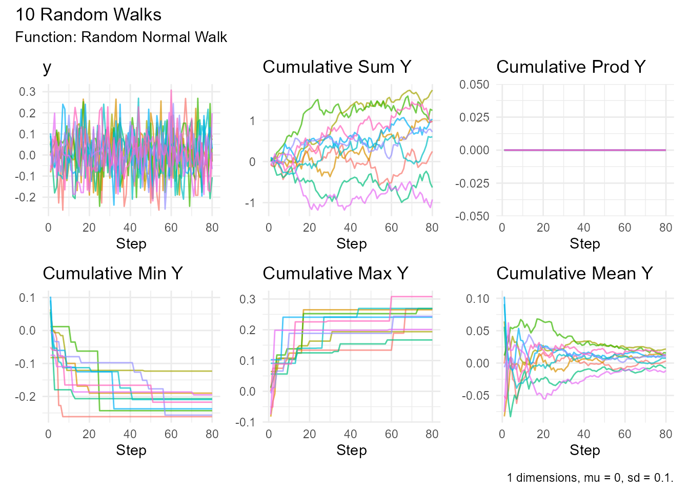

Line plot showing 10 random walks following a normal distribution, with steps on the x-axis and cumulative values on the y-axis. The walks fluctuate randomly around the starting value.

# With custom mean and SD
random_normal_walk(
  .num_walks = 5,
  .n = 200,
  .mu = 0.01,    # Slight upward drift
  .sd = 0.5,     # Lower volatility
  .initial_value = 100
) |> visualize_walks()

Line plot showing 5 random walks with custom mean and standard deviation parameters. The walks start at 100 and show an upward drift with lower volatility.

# 2D spatial walk
random_normal_walk(
  .num_walks = 3,
  .n = 500,
  .dimensions = 2
) |> visualize_walks()

Scatter plot showing 3 random walks in 2D space, with x-coordinate on the x-axis and y-coordinate on the y-axis. Each walk is represented by connected points forming a path through the 2D plane.

`random_normal_drift_walk()`

Random walk with deterministic drift component.

Function Signature:

random_normal_drift_walk(
  .num_walks = 25,
  .n = 100,
  .mu = 0,
  .sd = 1,
  .initial_value = 0,
  .dimensions = 1
)

Key Difference from random_normal_walk(): - .drift - Drift term added to each step (default: 0.1) - Adds explicit drift term: drift + random_step - More pronounced trending behavior - Better for modeling processes with clear directional movement

Example:

# Compare walks with and without drift
p1 <- random_normal_walk(.num_walks = 5, .mu = 0.1) |>
  visualize_walks(.pluck = "y") +
  labs(title = "Normal Walk")

p2 <- random_normal_drift_walk(.num_walks = 5, .mu = 0.1) |>
  visualize_walks(.pluck = "y") +
  labs(title = "Normal Walk with Drift")

p1 / p2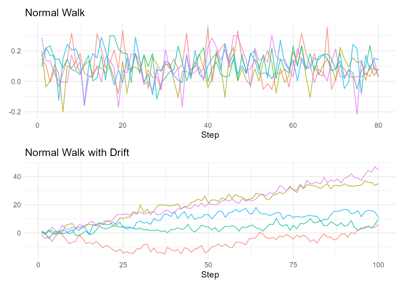

Two panel plot comparing normal walks with and without drift. The top panel shows walks with subtle drift, while the bottom panel shows walks with more pronounced trending behavior due to explicit drift term.

Brownian Motion

`brownian_motion()`

Standard Brownian motion (Wiener process) - the foundation of stochastic calculus.

Function Signature:

brownian_motion(
  .num_walks = 25,
  .n = 100,
  .delta_time = 1,
  .initial_value = 0,
  .dimensions = 1
)

Parameters: - .num_walks - Number of walks to generate (default: 25) - .n - Number of steps per walk (default: 100) - .delta_time - Time increment per step (default: 1) - .initial_value - Starting value for each walk (default: 0) - .dimensions - Number of dimensions (default: 1)

Mathematical Form:

Use Cases: - Financial mathematics (Black-Scholes model) - Physics (particle diffusion) - Signal processing (noise modeling)

Example:

# Standard Brownian motion
brownian_motion(.num_walks = 10) |>
  visualize_walks()

Line plot showing 10 standard Brownian motion paths. The paths start at zero and fluctuate randomly with continuous movements typical of Wiener processes.

# With drift and volatility
brownian_motion(
  .num_walks = 50,
  .n = 252,
  .delta_time = 0.05,
  .initial_value = 100
) |> visualize_walks(.alpha = 0.3)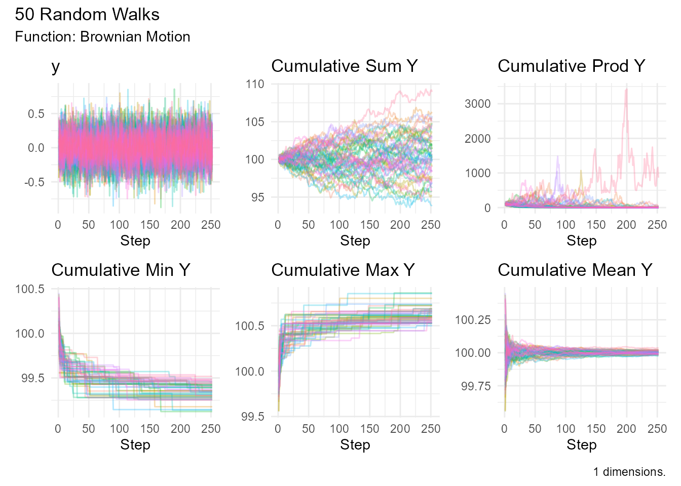

Line plot showing 50 Brownian motion paths with custom drift and volatility parameters. The paths start at 100 and show semi-transparent overlapping trajectories.

`geometric_brownian_motion()`

Geometric Brownian motion - the standard model for stock prices.

Function Signature:

geometric_brownian_motion(
  .num_walks = 25,
  .n = 100,
  .mu = 0,
  .sigma = 0.1,
  .initial_value = 100,
  .delta_time = 0.003,
  .dimensions = 1
)

Parameters: - .mu - Expected return (drift) - .sigma - Volatility

Mathematical Form:

dS(t) = μ S(t) dt + σ S(t) dW(t)
S(t) = S(0) exp((μ - σ²/2)t + σW(t))

Key Properties: - Always positive (can’t go below zero) - Log-normal distribution of prices - Percentage changes are normally distributed

Use Cases: - Stock price modeling - Option pricing - Asset allocation simulations - Monte Carlo risk analysis

Example:

# Model stock prices
stock_sim <- geometric_brownian_motion(
  .num_walks = 1000,
  .n = 252,        # Trading days in a year
  .mu = 0.08,      # 8% expected return
  .sigma = 0.25,   # 25% volatility
  .initial_value = 100
)

# Visualize scenarios
stock_sim |> visualize_walks(.alpha = 0.1)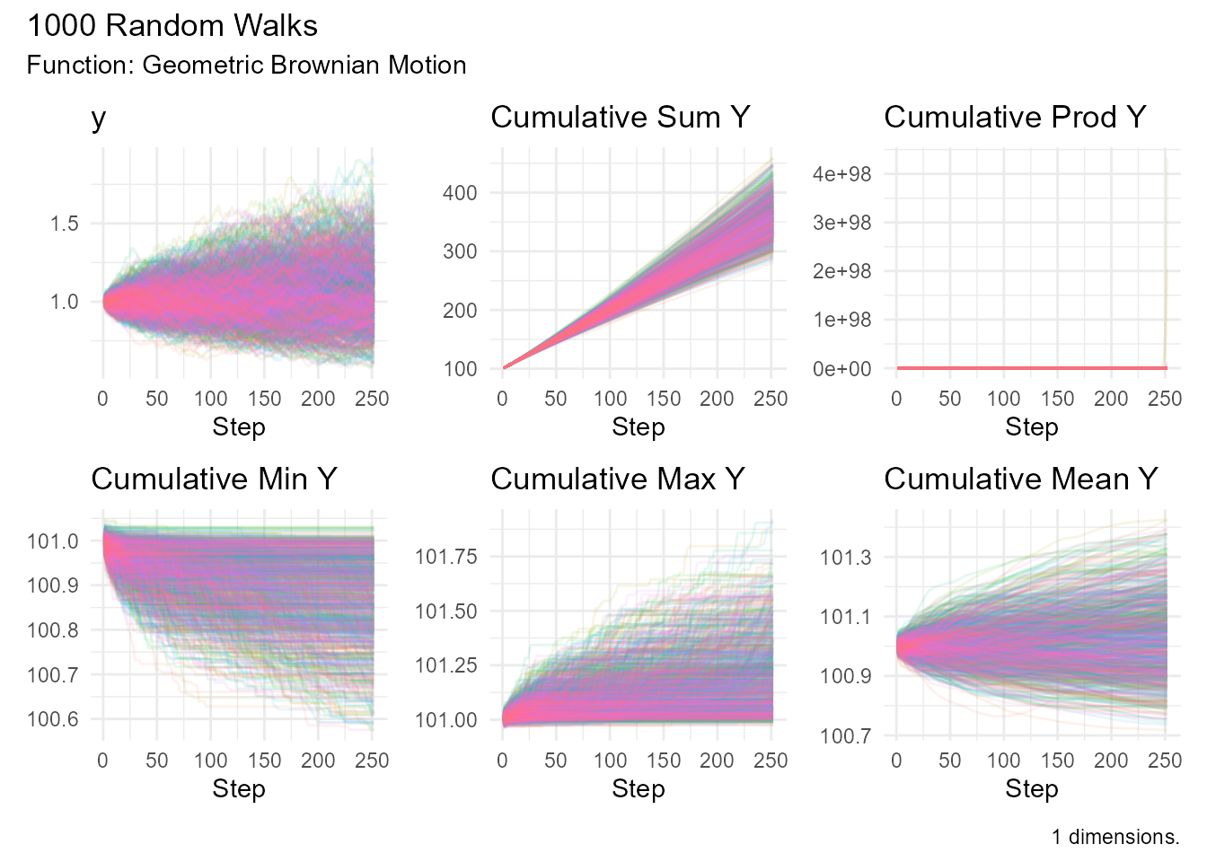

Line plot showing 1000 semi-transparent stock price simulation paths using geometric Brownian motion. All paths start at 100 and spread out over time, remaining positive throughout.

# Analyze outcomes
stock_sim |>
  summarize_walks(.value = cum_prod_y, .group_var = walk_number) |>
  summarize(
    median_price = median(max_val),
    prob_profit = mean(max_val > 100),
    prob_loss_50 = mean(min_val < 50)
  )

Beta Distribution

`random_beta_walk()`

Random walk based on the beta distribution (bounded between 0 and 1).

Function Signature:

random_beta_walk(
  .num_walks = 25,
  .n = 100,
  .shape1 = 2,
  .shape2 = 2,
  .ncp = 0,
  .initial_value = 0,
  .samp = TRUE,
  .replace = TRUE,
  .sample_size = 0.8,
  .dimensions = 1
)

Parameters: - .shape1 - First shape parameter (α) - .shape2 - Second shape parameter (β) - .ncp - Non-centrality parameter (default: 0)

Properties: - Steps are bounded: 0 ≤ step ≤ 1 - Flexible shapes (uniform, U-shaped, bell-shaped) - Mean = α / (α + β) - Variance = (α β) / ((α + β)² (α + β + 1))

Shape Guide: - shape1 = 1, shape2 = 1: Uniform (0,1) - shape1 = 2, shape2 = 2: Symmetric, bell-shaped - shape1 = 2, shape2 = 5: Right-skewed - shape1 = 5, shape2 = 2: Left-skewed

Use Cases: - Modeling proportions or percentages - Bounded processes (e.g., utilization rates) - Success rates over time

Example:

# Symmetric beta walk
random_beta_walk(
  .num_walks = 10,
  .shape1 = 2,
  .shape2 = 2
) |> visualize_walks()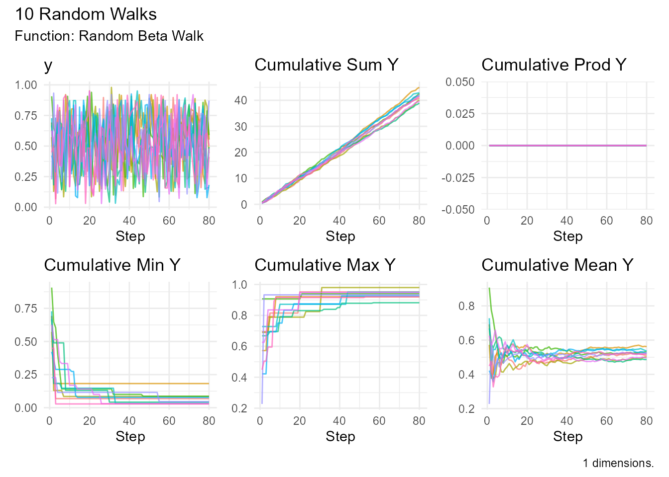

Line plot showing 10 random walks following a symmetric beta distribution with shape parameters 2 and 2. The walks fluctuate with steps bounded between 0 and 1.

# Right-skewed (toward 0)
random_beta_walk(
  .num_walks = 10,
  .shape1 = 2,
  .shape2 = 5
) |> visualize_walks()

Line plot showing 10 random walks following a right-skewed beta distribution with shape parameters 2 and 5. The walks show a tendency toward lower values.

# Compare different shapes
p1 <- random_beta_walk(.shape1 = 1, .shape2 = 1) |>
  visualize_walks(.pluck = "y")
p2 <- random_beta_walk(.shape1 = 2, .shape2 = 5) |>
  visualize_walks(.pluck = "y")
p1 / p2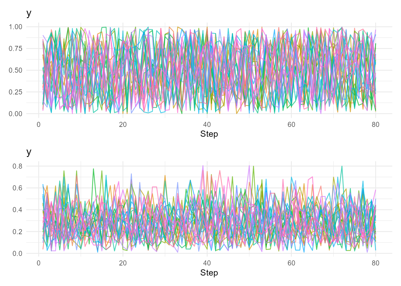

Two panel plot comparing beta distributions with different shape parameters. The top panel shows uniform (1,1) beta walks, while the bottom panel shows right-skewed (2,5) beta walks.

Cauchy Distribution

`random_cauchy_walk()`

Random walk with heavy tails - extreme values are much more common than in normal distribution.

Function Signature:

random_cauchy_walk(
  .num_walks = 25,
  .n = 100,
  .location = 0,
  .scale = 1,
  .initial_value = 0,
  .samp = TRUE,
  .replace = TRUE,
  .sample_size = 0.8,
  .dimensions = 1
)

Parameters: - .location - Location parameter (median) - .scale - Scale parameter (spread)

Properties: - No defined mean or variance! - Heavy tails (high probability of extreme values) - Symmetric around location - Much more volatile than normal distribution

Use Cases: - Modeling extreme events - Financial crises simulation - Physics (resonance phenomena) - Robust statistics demonstrations

Example:

# Standard Cauchy walk
random_cauchy_walk(.num_walks = 10) |>
  visualize_walks()

Line plot showing 10 random walks following a Cauchy distribution. The walks exhibit extreme volatility with large jumps due to the heavy-tailed distribution.

# Compare with normal walk
p1 <- random_normal_walk(.num_walks = 5, .sd = 1) |>
  visualize_walks(.pluck = "y") +
  labs(title = "Normal Walk")

p2 <- random_cauchy_walk(.num_walks = 5, .scale = 1) |>
  visualize_walks(.pluck = "y") +
  labs(title = "Cauchy Walk (Heavy Tails)")

p1 / p2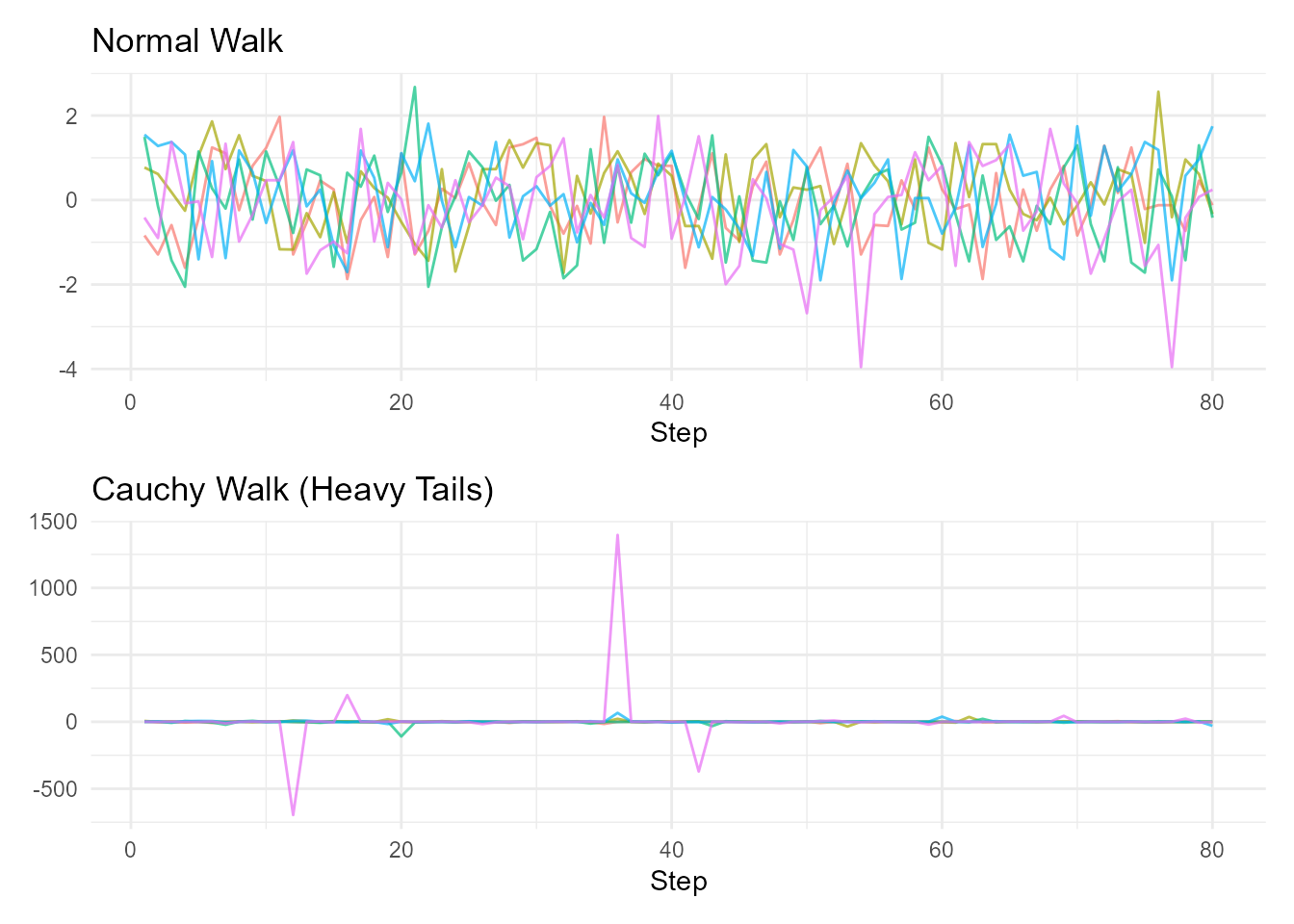

Two panel plot comparing normal walks (top) versus Cauchy walks (bottom). The Cauchy walks show much more extreme movements and larger fluctuations due to heavy tails.

Chi-Squared Distribution

`random_chisquared_walk()`

Random walk based on chi-squared distribution (always positive).

Function Signature:

random_chisquared_walk(
  .num_walks = 25,
  .n = 100,
  .df = 5,
  .ncp = 0,
  .initial_value = 0,
  .samp = TRUE,
  .replace = TRUE,
  .sample_size = 0.8,
  .dimensions = 1
)

Parameters: - .df - Degrees of freedom - .ncp - Non-centrality parameter (default: 0)

Properties: - Steps are always positive - Right-skewed (especially for low df) - Mean = df - Variance = 2df

Use Cases: - Goodness-of-fit tests - Variance estimation - Quality control - Reliability engineering

Example:

# Low df (very skewed)
random_chisquared_walk(.num_walks = 10, .df = 1) |>
  visualize_walks()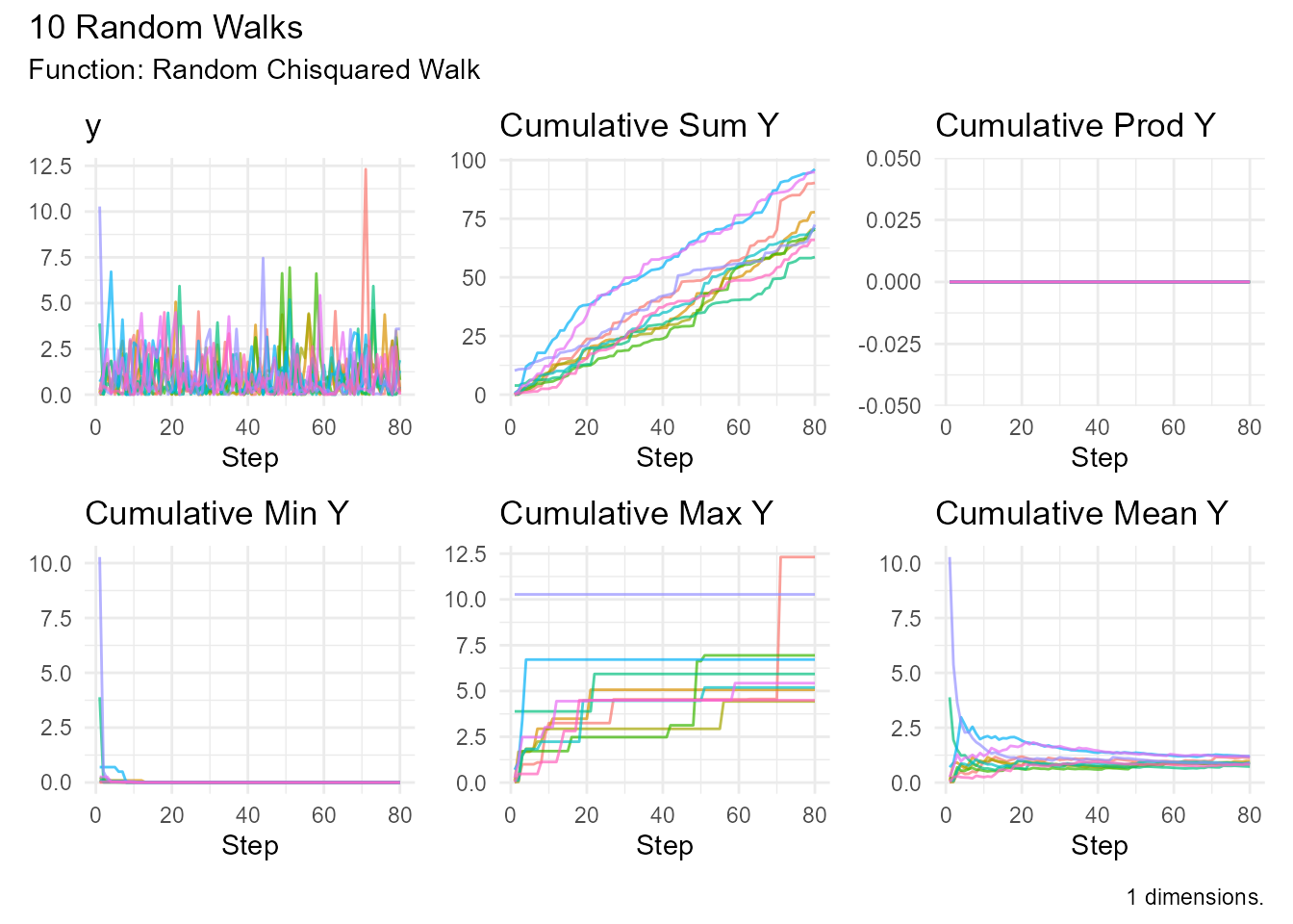

Line plot showing 10 random walks following a chi-squared distribution with 1 degree of freedom. The walks are strongly right-skewed with always positive steps.

# Higher df (more symmetric)
random_chisquared_walk(.num_walks = 10, .df = 10) |>
  visualize_walks()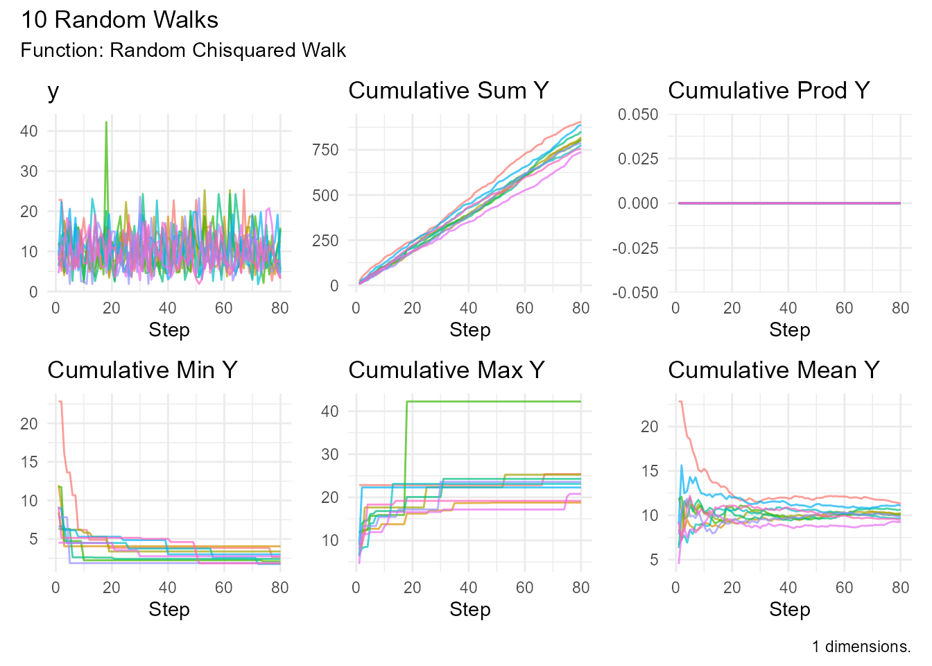

Line plot showing 10 random walks following a chi-squared distribution with 10 degrees of freedom. The walks are more symmetric than the low df case but still show positive steps only.

Exponential Distribution

`random_exponential_walk()`

Random walk with exponentially distributed steps (memoryless property).

Function Signature:

random_exponential_walk(
  .num_walks = 25,
  .n = 100,
  .rate = 1,
  .initial_value = 0,
  .samp = TRUE,
  .replace = TRUE,
  .sample_size = 0.8,
  .dimensions = 1
)

Parameters: - .rate - Rate parameter (λ)

Properties: - Steps are always positive - Memoryless property - Mean = 1/rate - Variance = 1/rate²

Use Cases: - Time between events (queuing theory) - Lifetime modeling - Radioactive decay - Poisson process intervals

Example:

# Standard exponential
random_exponential_walk(.num_walks = 10) |>
  visualize_walks()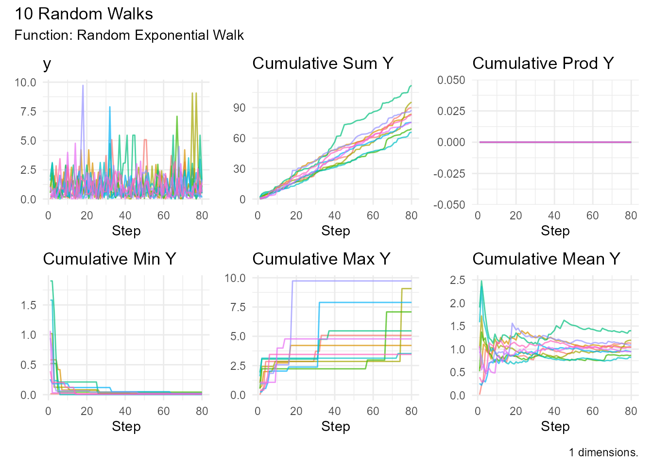

Line plot showing 10 random walks following a standard exponential distribution. The walks increase monotonically with always positive steps.

# Fast rate (smaller steps)
random_exponential_walk(.num_walks = 10, .rate = 5) |>
  visualize_walks()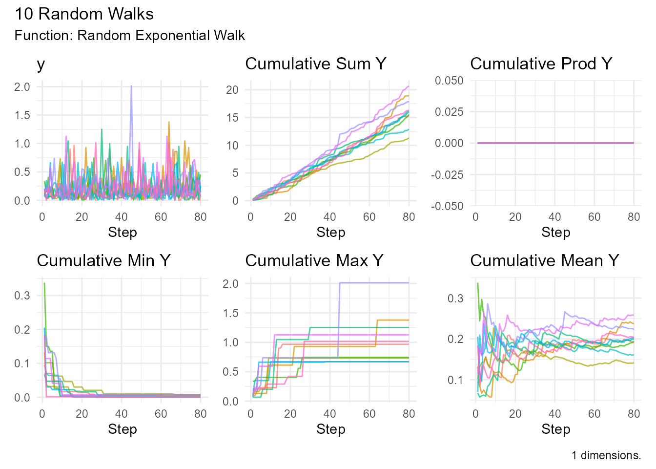

Line plot showing 10 random walks with fast exponential rate (5). The walks show smaller steps compared to the standard rate.

# Slow rate (larger steps)
random_exponential_walk(.num_walks = 10, .rate = 0.5) |>
  visualize_walks()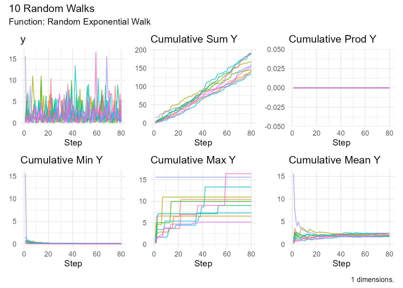

Line plot showing 10 random walks with slow exponential rate (0.5). The walks show larger steps compared to the standard rate.

F Distribution

`random_f_walk()`

Random walk based on F-distribution (ratio of chi-squared variables).

Function Signature:

random_f_walk(
  .num_walks = 25,
  .n = 100,
  .df1 = 5,
  .df2 = 5,
  .ncp = NULL,
  .initial_value = 0,
  .samp = TRUE,
  .replace = TRUE,
  .sample_size = 0.8,
  .dimensions = 1
)

Parameters: - .df1 - Numerator degrees of freedom - .df2 - Denominator degrees of freedom - .ncp - Non-centrality parameter

Use Cases: - ANOVA - Variance ratio tests - Model comparison

Example:

random_f_walk(.num_walks = 10, .df1 = 5, .df2 = 10) |>
  visualize_walks()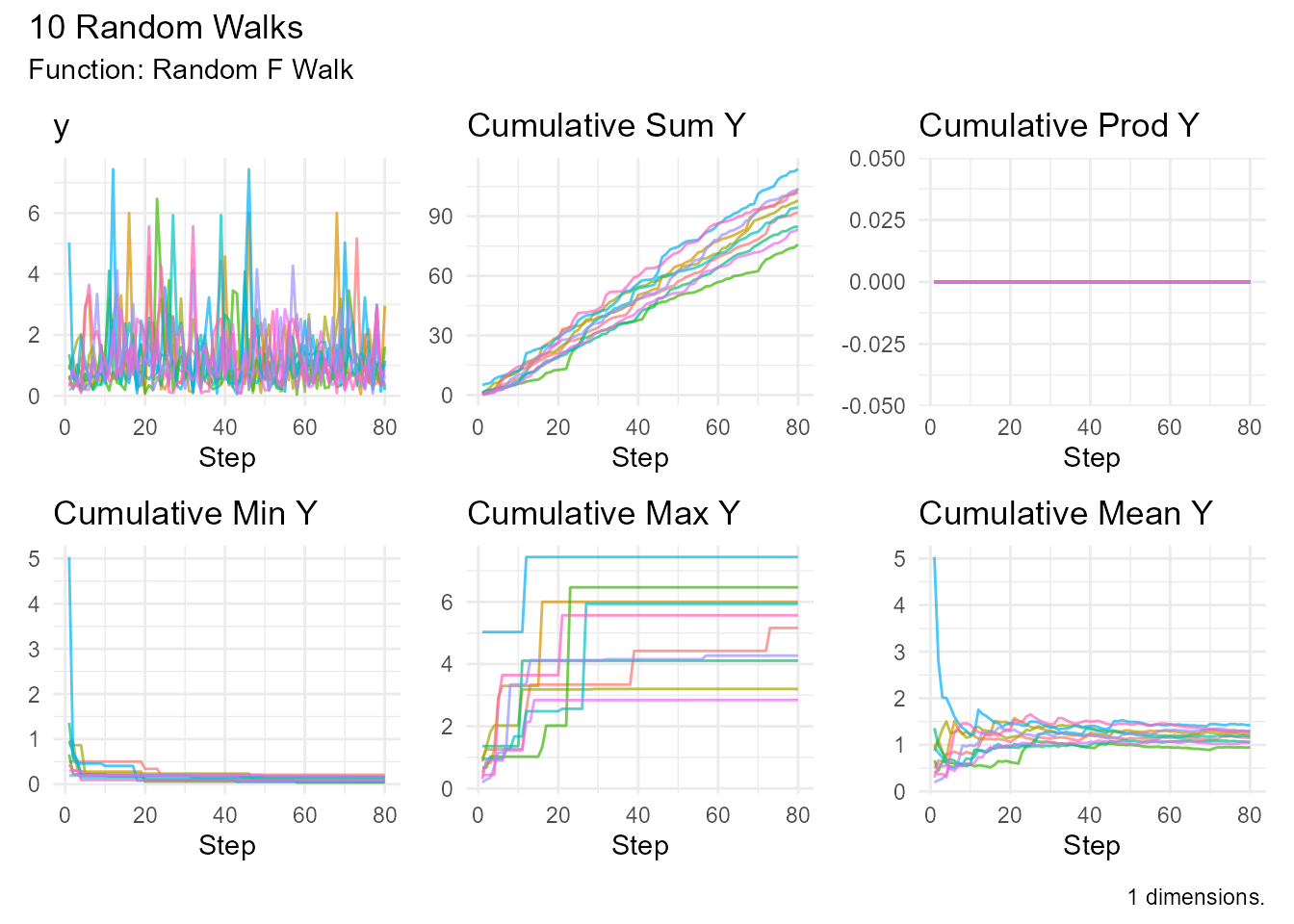

Line plot showing 10 random walks following an F-distribution with 5 and 10 degrees of freedom. The walks show right-skewed behavior typical of F-distributions.

Gamma Distribution

`random_gamma_walk()`

Flexible distribution for positive values.

Function Signature:

random_gamma_walk(
  .num_walks = 25,
  .n = 100,
  .shape = 1,
  .scale = 1,
  .rate = NULL,
  .initial_value = 0,
  .samp = TRUE,
  .replace = TRUE,
  .sample_size = 0.8,
  .dimensions = 1
)

Parameters: - .shape - Shape parameter (k) - .rate - Rate parameter (β) - .scale - Scale parameter (1/rate)

Properties: - Steps always positive - Flexible shapes - Mean = shape/rate - Variance = shape/rate²

Use Cases: - Waiting times - Rainfall modeling - Insurance claims - Reliability analysis

Example:

# Different shape parameters
random_gamma_walk(.num_walks = 10, .shape = 1, .rate = 1) |>
  visualize_walks()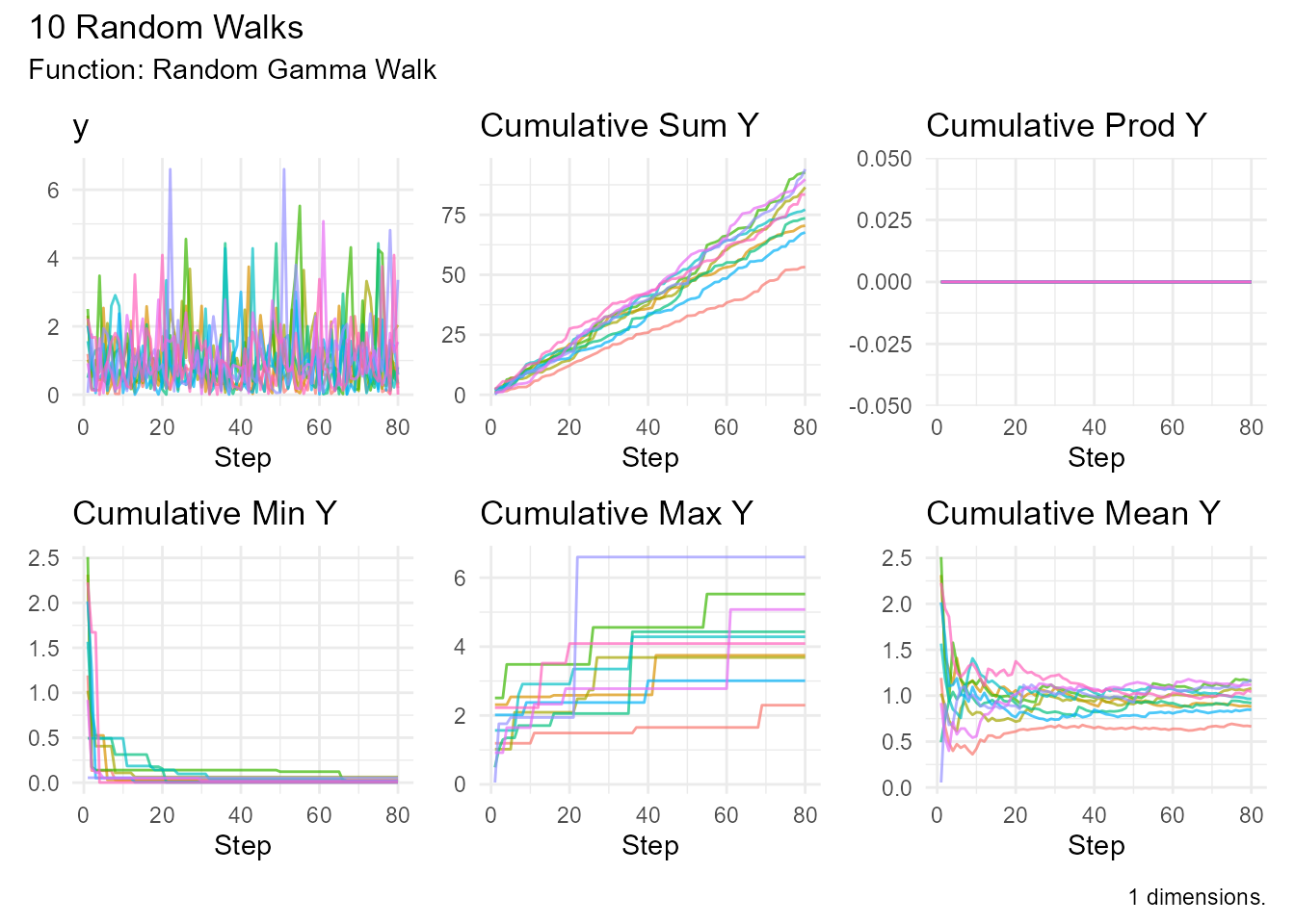

Line plot showing 10 random walks following a gamma distribution with shape parameter 1. The walks show exponential-like behavior with always positive steps.

random_gamma_walk(.num_walks = 10, .shape = 5, .rate = 1) |>
  visualize_walks()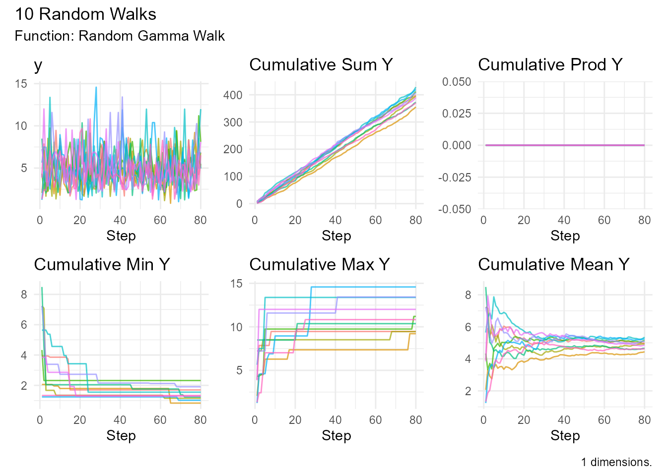

Line plot showing 10 random walks following a gamma distribution with shape parameter 5. The walks show more symmetric behavior compared to shape 1.

Log-Normal Distribution

`random_lognormal_walk()`

Random walk where log of steps is normally distributed.

Function Signature:

random_lognormal_walk(
  .num_walks = 25,
  .n = 100,
  .meanlog = 0,
  .sdlog = 1,
  .initial_value = 0,
  .samp = TRUE,
  .replace = TRUE,
  .sample_size = 0.8,
  .dimensions = 1
)

Parameters: - .meanlog - Mean of log - .sdlog - Standard deviation of log

Properties: - Steps always positive - Right-skewed - Multiplicative processes

Use Cases: - Income distributions - File sizes - Particle sizes - Stock prices (alternative to GBM)

Example:

random_lognormal_walk(.num_walks = 10) |>
  visualize_walks()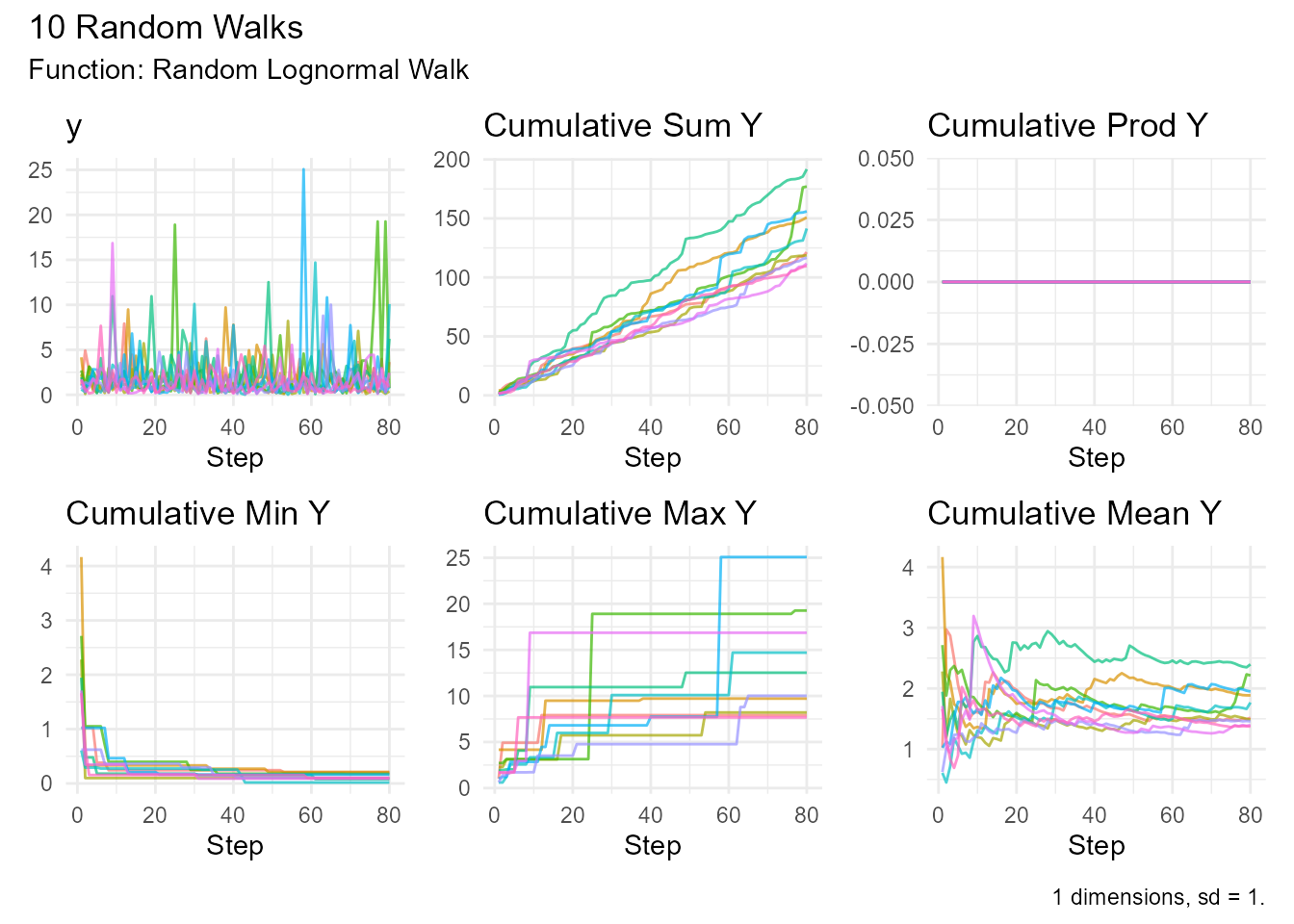

Line plot showing 10 random walks following a log-normal distribution. The walks are right-skewed with always positive steps typical of log-normal distributions.

Logistic Distribution

`random_logistic_walk()`

Random walk with logistic distribution (heavier tails than normal).

Function Signature:

random_logistic_walk(
  .num_walks = 25,
  .n = 100,
  .location = 0,
  .scale = 1,
  .initial_value = 0,
  .samp = TRUE,
  .replace = TRUE,
  .sample_size = 0.8,
  .dimensions = 1
)

Use Cases: - Growth models - Binary classification - Neural networks

Example:

random_logistic_walk(.num_walks = 10) |>
  visualize_walks()

Line plot showing 10 random walks following a logistic distribution. The walks have symmetric fluctuations with slightly heavier tails than normal distribution.

Student’s t Distribution

`random_t_walk()`

Random walk with t-distribution (adjustable tail heaviness).

Function Signature:

random_t_walk(
  .num_walks = 25,
  .n = 100,
  .df = 5,
  .initial_value = 0,
  .ncp = 0,
  .samp = TRUE,
  .replace = TRUE,
  .sample_size = 0.8,
  .dimensions = 1
)

Parameters: - .df - Degrees of freedom (controls tail heaviness) - .ncp - Non-centrality parameter

Properties: - Heavier tails than normal (for low df) - Approaches normal as df → ∞ - Mean = 0 (if df > 1) - Variance = df/(df-2) (if df > 2)

Use Cases: - Robust statistics - Small sample inference - Financial returns modeling

Example:

# Heavy tails (df = 3)
random_t_walk(.num_walks = 10, .df = 3) |>
  visualize_walks()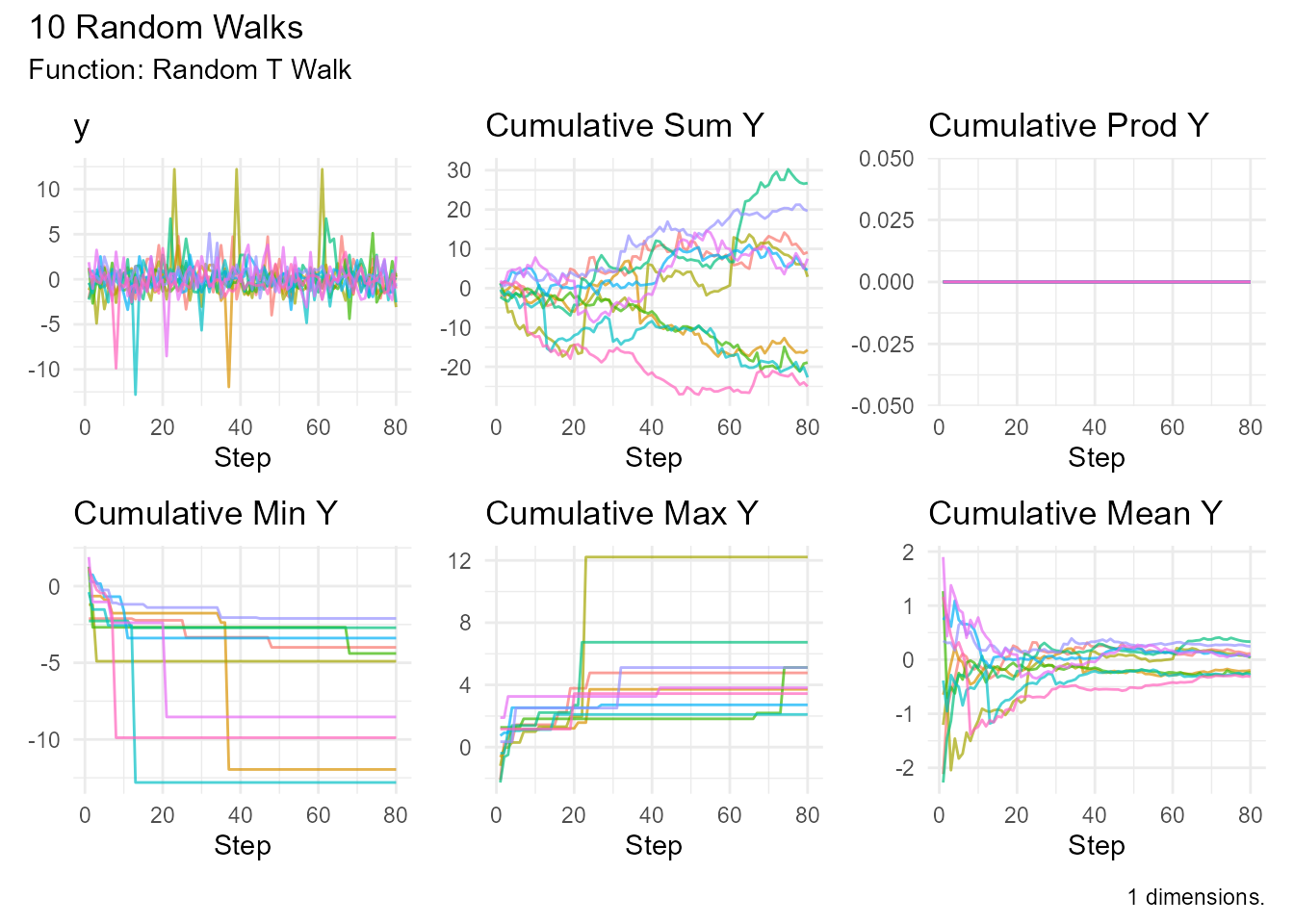

Line plot showing 10 random walks following a t-distribution with 3 degrees of freedom. The walks show heavy tails with occasional large jumps.

# Nearly normal (df = 30)
random_t_walk(.num_walks = 10, .df = 30) |>
  visualize_walks()

Line plot showing 10 random walks following a t-distribution with 30 degrees of freedom. The walks closely resemble normal walks with lighter tails.

Uniform Distribution

`random_uniform_walk()`

Random walk with uniformly distributed steps.

Function Signature:

random_uniform_walk(
  .num_walks = 25,
  .n = 100,
  .min = 0,
  .max = 1,
  .initial_value = 0,
  .samp = TRUE,
  .replace = TRUE,
  .sample_size = 0.8,
  .dimensions = 1
)

Parameters: - .min - Minimum value - .max - Maximum value

Properties: - All values equally likely - Mean = (min + max) / 2 - Variance = (max - min)² / 12

Use Cases: - Modeling equal probabilities - Random sampling - Monte Carlo simulations

Example:

# Symmetric around 0
random_uniform_walk(.num_walks = 10, .min = -1, .max = 1) |>
  visualize_walks()

Line plot showing 10 random walks with uniformly distributed steps between -1 and 1. The walks show bounded steps with all values equally likely.

Weibull Distribution

`random_weibull_walk()`

Random walk with Weibull distribution (flexible lifetime model).

Function Signature:

random_weibull_walk(
  .num_walks = 25,
  .n = 100,
  .shape = 1,
  .scale = 1,
  .initial_value = 0,
  .samp = TRUE,
  .replace = TRUE,
  .sample_size = 0.8,
  .dimensions = 1
)

Parameters: - .shape - Shape parameter (k) - .scale - Scale parameter (λ)

Properties: - Steps always positive - shape < 1: Decreasing failure rate - shape = 1: Constant failure rate (exponential) - shape > 1: Increasing failure rate

Use Cases: - Reliability engineering - Survival analysis - Wind speed modeling - Materials science

Example:

# Different shape parameters
random_weibull_walk(.num_walks = 10, .shape = 0.5) |>
  visualize_walks()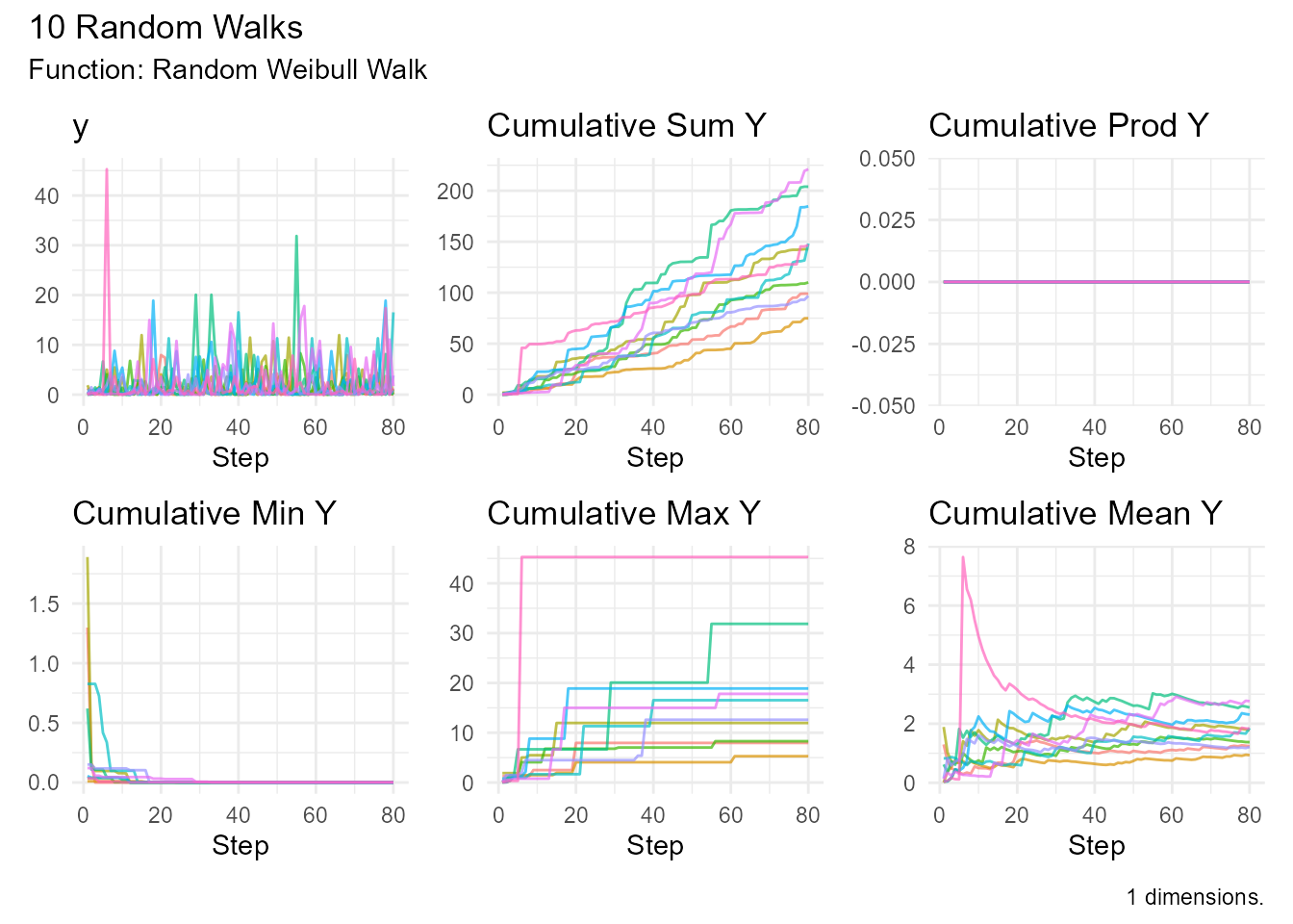

Line plot showing 10 random walks following a Weibull distribution with shape parameter 0.5. The walks show decreasing failure rate behavior with always positive steps.

random_weibull_walk(.num_walks = 10, .shape = 2) |>
  visualize_walks()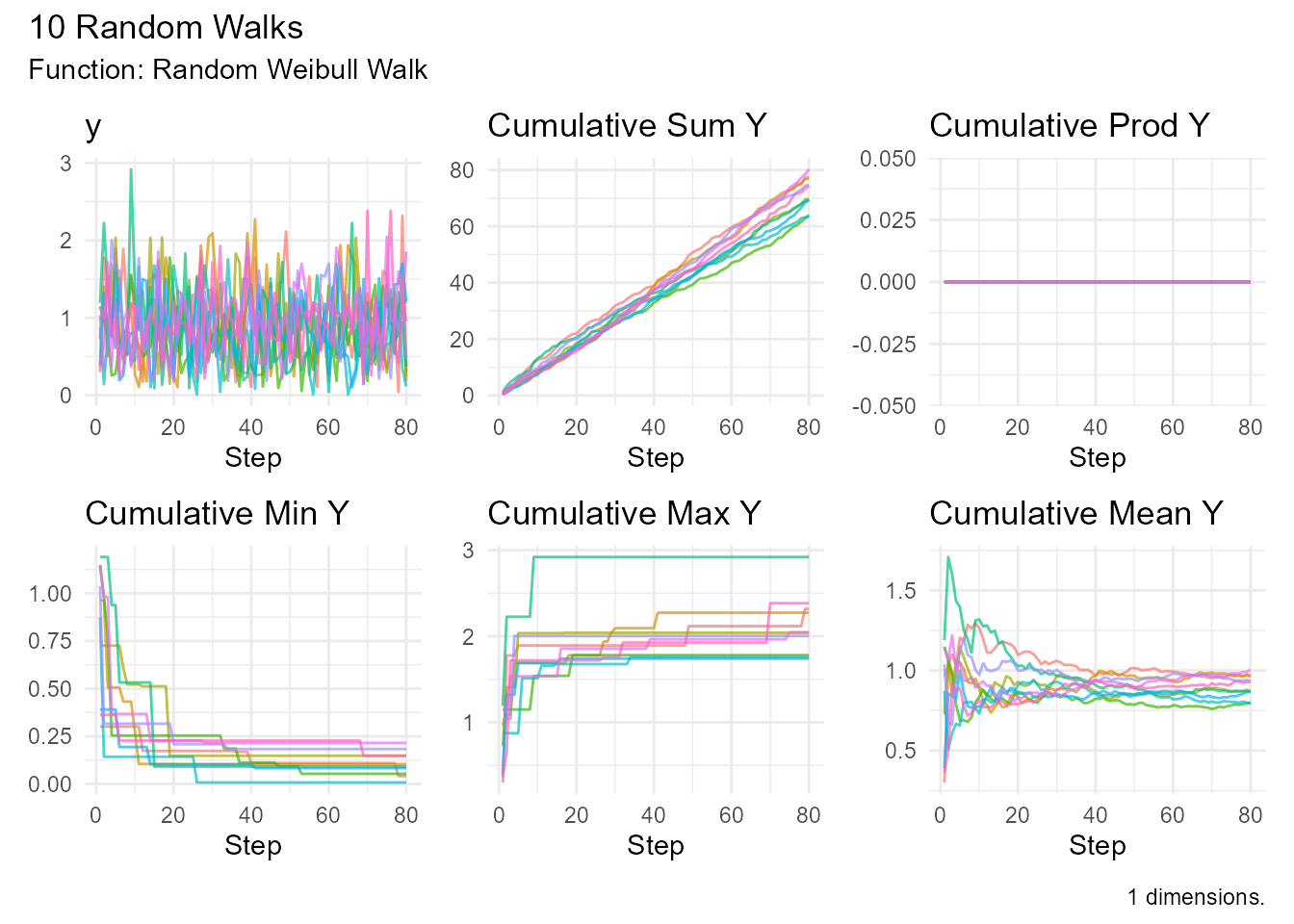

Line plot showing 10 random walks following a Weibull distribution with shape parameter 2. The walks show increasing failure rate behavior.

Comparison Guide

When to Use Each Distribution

Distribution	Use When…	Key Property
Normal	General modeling, natural phenomena	Symmetric, bell-shaped
Brownian Motion	Continuous stochastic processes	Foundation of stochastic calculus
Geometric Brownian	Stock prices, always positive	Log-normal, multiplicative
Beta	Bounded processes (0-1)	Flexible shapes, bounded
Cauchy	Extreme events, heavy tails	No mean/variance
Chi-Squared	Sum of squares, variance tests	Right-skewed, positive
Exponential	Time between events	Memoryless property
F	Variance ratios	Ratio of chi-squared
Gamma	Positive values, waiting times	Flexible, positive
Log-Normal	Multiplicative processes	Right-skewed, positive
Logistic	S-curves, classification	Heavier tails than normal
Student’s t	Robust modeling, small samples	Adjustable tail heaviness
Uniform	Equal probabilities	All values equally likely
Weibull	Reliability, survival	Flexible failure rates

Tail Behavior

Light Tails (fewer extreme values): - Uniform

Medium Tails: - Normal - Exponential - Gamma (shape > 1)

Heavy Tails (more extreme values): - Logistic - Student’s t (low df) - Cauchy (extreme)

Symmetry

Symmetric: - Normal - Brownian Motion - Cauchy - Logistic - Student’s t - Uniform

Right-Skewed (tail extends right): - Beta (depends on parameters) - Chi-Squared - Exponential - F - Gamma - Log-Normal - Weibull (depends on shape)

Next Steps

Discrete Distribution Generators - Explore discrete distributions
Multi-Dimensional Walks - Work in 2D and 3D
Visualization Guide - Create beautiful plots
Use Cases and Examples - Real-world applications

Need help choosing? Check out the FAQ or Use Cases for guidance!

Table of Contents

Common Parameters

Normal Distribution

random_normal_walk()

random_normal_drift_walk()

Brownian Motion

brownian_motion()

geometric_brownian_motion()

Beta Distribution

random_beta_walk()

Cauchy Distribution

random_cauchy_walk()

Chi-Squared Distribution

random_chisquared_walk()

Exponential Distribution

random_exponential_walk()

F Distribution

random_f_walk()

Gamma Distribution

random_gamma_walk()

Log-Normal Distribution

random_lognormal_walk()

Logistic Distribution

random_logistic_walk()

Student’s t Distribution

random_t_walk()

Uniform Distribution

random_uniform_walk()

Weibull Distribution

random_weibull_walk()

Comparison Guide

When to Use Each Distribution

Tail Behavior

Symmetry

Next Steps

`random_normal_walk()`

`random_normal_drift_walk()`

`brownian_motion()`

`geometric_brownian_motion()`

`random_beta_walk()`

`random_cauchy_walk()`

`random_chisquared_walk()`

`random_exponential_walk()`

`random_f_walk()`

`random_gamma_walk()`

`random_lognormal_walk()`

`random_logistic_walk()`

`random_t_walk()`

`random_uniform_walk()`

`random_weibull_walk()`