Overview
To view the full wiki click here: Full TidyDensity Wiki
TidyDensity is a comprehensive R package that makes working with random numbers and probability distributions easy, intuitive, and tidy. Whether you’re simulating data, exploring distributions, or performing statistical analysis, TidyDensity provides a unified interface that integrates seamlessly with the tidyverse ecosystem.
Key Features
- 35+ Probability Distributions: Generate random data from a wide variety of continuous and discrete distributions
- Tidy Output: All functions return tibbles with a consistent, predictable structure
-
Rich Metadata: Each distribution includes density (
d_), probability (p_), quantile (q_), and random generation (r_) components - Beautiful Visualizations: Built-in plotting functions with support for multiple plot types
- Parameter Estimation: Estimate distribution parameters from empirical data using MLE, MME, and MVUE methods
- Bootstrap Analysis: Perform bootstrap resampling with integrated plotting and analysis tools
- Mixture Models: Create and analyze mixture distributions
- Interactive Plots: Generate interactive visualizations with plotly integration
Installation
Install the released version from CRAN:
install.packages("TidyDensity")Or install the development version from GitHub:
# install.packages("devtools")
devtools::install_github("spsanderson/TidyDensity")
Quick Start
Generate random data from a normal distribution and visualize it:
library(TidyDensity)
library(dplyr)
library(ggplot2)

# Generate data from normal distribution
tn <- tidy_normal(.n = 100, .mean = 0, .sd = 1, .num_sims = 6)

# View the tibble structure
tn
#> # A tibble: 600 × 7
#>    sim_number     x       y    dx       dy      p       q
#>    <fct>      <int>   <dbl> <dbl>    <dbl>  <dbl>   <dbl>
#>  1 1              1 -0.626  -3.51 0.000235 0.266  -0.626
#>  2 1              2  0.184  -3.37 0.000617 0.573   0.184
#>  3 1              3 -0.836  -3.22 0.00147  0.202  -0.836
#>  4 1              4  1.60   -3.07 0.00322  0.945   1.60
#> # ... with 596 more rows
All tidy_ distribution functions return a tibble with the following columns:
-
sim_number: Simulation identifier -
x: Index of generated point -
y: The randomly generated value -
dx: Density function x-values -
dy: Density function y-values (PDF) -
p: Cumulative probability (CDF) -
q: Quantile values
Visualization
TidyDensity includes tidy_autoplot() for quick, publication-ready visualizations:
# Density plot
tidy_autoplot(tn, .plot_type = "density")

# Quantile plot
tidy_autoplot(tn, .plot_type = "quantile")

# Probability plot
tidy_autoplot(tn, .plot_type = "probability")

# QQ plot
tidy_autoplot(tn, .plot_type = "qq")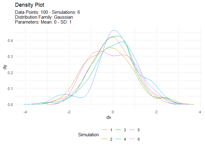
When simulating many distributions, the legend is automatically hidden for clarity:
tn <- tidy_normal(.n = 100, .num_sims = 20)
tidy_autoplot(tn, .plot_type = "density")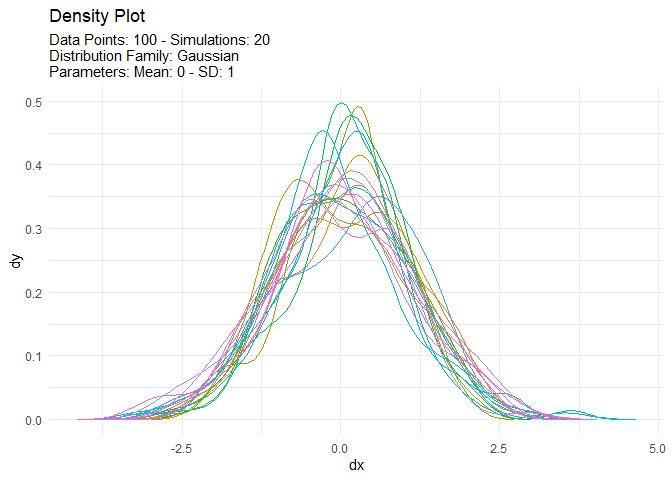
Supported Distributions
TidyDensity supports 35+ probability distributions:
Continuous Distributions
- Normal Family: Normal, Log-Normal, Inverse Normal
- Exponential Family: Exponential, Inverse Exponential
- Gamma Family: Gamma, Inverse Gamma
- Beta Family: Beta, Generalized Beta
- Pareto Family: Pareto, Inverse Pareto, Single Parameter Pareto, Generalized Pareto
- Weibull Family: Weibull, Inverse Weibull
- Burr Family: Burr, Inverse Burr
- Other: Cauchy, Chi-Square, F-Distribution, t-Distribution, Logistic, Paralogistic, Triangular, Uniform
Discrete Distributions
- Bernoulli
- Binomial
- Zero-Truncated Binomial
- Geometric
- Zero-Truncated Geometric
- Hypergeometric
- Negative Binomial
- Poisson
- Zero-Truncated Poisson
Each distribution has a corresponding tidy_*() function, e.g., tidy_beta(), tidy_gamma(), tidy_poisson().
Advanced Features
Parameter Estimation
Estimate distribution parameters from empirical data:
# Generate sample data
x <- mtcars$mpg

# Estimate normal distribution parameters
est <- util_normal_param_estimate(x, .auto_gen_empirical = TRUE)

# View parameter estimates
est$parameter_tbl
#> # A tibble: 2 × 7
#>   dist_type samp_size   min   max  mean method   shape_est
#>   <chr>         <int> <dbl> <dbl> <dbl> <chr>        <dbl>
#> 1 Gaussian         32  10.4  33.9  20.1 MLE/MME      6.03
#> 2 Gaussian         32  10.4  33.9  20.1 MVUE         6.10

# Compare empirical data with fitted distribution
est$combined_data_tbl |>
  tidy_combined_autoplot()
Bootstrap Analysis
Perform bootstrap resampling for robust statistical inference:
# Bootstrap resampling
bs <- tidy_bootstrap(mtcars$mpg, .num_sims = 2000)

# Bootstrap statistics
bootstrap_stat <- tidy_bootstrap(mtcars$mpg) |>
  bootstrap_unnest_tbl() |>
  summarise(
    mean_est = mean(y),
    sd_est = sd(y),
    ci_lower = quantile(y, 0.025),
    ci_upper = quantile(y, 0.975)
  )
Mixture Models
Create mixture distributions by combining multiple distributions:
# Create a mixture of two normal distributions
mix <- tidy_mixture_density(
  .tbl_list = list(
    tidy_normal(.n = 100, .mean = -2, .sd = 0.5),
    tidy_normal(.n = 100, .mean = 2, .sd = 0.5)
  ),
  .mixture_type = "add"
)

tidy_autoplot(mix, .plot_type = "density")
Empirical Distributions
Work directly with your own data:
# Create empirical distribution from data
emp <- tidy_empirical(mtcars$mpg, .num_sims = 5)

# Plot empirical distribution
tidy_autoplot(emp, .plot_type = "density")
Multiple Distribution Comparison
Compare multiple distributions with different parameters:
# Create multiple simulations with different parameters
multi <- tidy_multi_single_dist(
  .tidy_dist = "tidy_normal",
  .param_list = list(
    list(.n = 100, .mean = 0, .sd = 1),
    list(.n = 100, .mean = 0, .sd = 2),
    list(.n = 100, .mean = 2, .sd = 1)
  )
)

tidy_autoplot(multi, .plot_type = "density")Contributing
Contributions are welcome! Here’s how you can help:
- 🐛 Report bugs or request features via GitHub Issues
- 📝 Submit pull requests for bug fixes or new features
- 📖 Improve documentation or add examples
- ⭐ Star the repository to show your support
Please follow our Code of Conduct when participating in this project.
Getting Help
- 📖 Read the documentation
- 🐛 Report bugs at GitHub Issues
- 💬 Ask questions on GitHub Discussions
License
MIT License - see LICENSE.md for details