Introduction

Time series models are a powerful tool for forecasting future values of a time-dependent variable. These models are commonly used in a variety of fields, including finance, economics, and engineering, to predict future outcomes based on past data.

One important aspect of time series modeling is the ability to simulate model forecasts. This allows us to evaluate the performance of different forecasting methods and to compare the results of different models. Simulating forecasts also allows us to assess the uncertainty associated with our predictions, which can be especially useful when making important decisions based on the forecast.

There are several benefits to simulating time series model forecasts:

Improved accuracy: By simulating forecasts, we can identify the best forecasting method for a given time series and optimize its parameters. This can lead to more accurate forecasts, especially for long-term predictions.
Enhanced understanding: Simulating forecasts helps us to understand how different factors, such as seasonality and trend, affect the prediction. This understanding can inform our decision-making and allow us to make more informed predictions.
Improved communication: Simulating forecasts allows us to present the uncertainty associated with our predictions, which can be useful for communicating the potential risks and benefits of different courses of action.

The R package {healthyR.ts} includes a function called ts_forecast_simulator() that can be used to simulate time series model forecasts. This function allows users to specify the forecasting method, the number of simulations to run, and the length of the forecast horizon. It also provides options for visualizing the results, including plots of the forecast distribution and summary statistics such as the mean and standard deviation of the forecasts.

In summary, simulating time series model forecasts is a valuable tool for improving the accuracy and understanding of our predictions, as well as for communicating the uncertainty associated with these forecasts. The ts_forecast_simulator() function in the {healthyR.ts} package is a useful tool for performing these simulations in R.

Function

Let’s take a look at the full function call.

ts_forecast_simulator(
  .model,
  .data,
  .ext_reg = NULL,
  .frequency = NULL,
  .bootstrap = TRUE,
  .horizon = 4,
  .iterations = 25,
  .sim_color = "steelblue",
  .alpha = 0.05
)

Now let’s take a look at the arguments that get provided to the parameters.

.model - A forecasting model of one of the following from the forecast package:
- Arima
- auto.arima
- ets
- nnetar
- Arima() with xreg
.data - The data that is used for the .model parameter. This is used with timetk::tk_index()
.ext_reg - A tibble or matrix of future xregs that should be the same length as the horizon you want to forecast.
.frequency - This is for the conversion of an internal table and should match the time frequency of the data.
.bootstrap - A boolean value of TRUE/FALSE. From forecast::simulate.Arima() Do simulation using resampled errors rather than normally distributed errors.
.horizon - An integer defining the forecast horizon.
.iterations - An integer, set the number of iterations of the simulation.
.sim_color - Set the color of the simulation paths lines.
.alpha - Set the opacity level of the simulation path lines.

Great, now let’s take a look at examples.

Examples

library(healthyR.ts)
library(forecast)

fit <- auto.arima(AirPassengers)
data_tbl <- ts_to_tbl(AirPassengers)

# Simulate 50 possible forecast paths, with .horizon of 12 months
output <- ts_forecast_simulator(
  .model        = fit
  , .horizon    = 12
  , .iterations = 50
  , .data       = data_tbl
)

Ok, so now we have our output object, which is a list object. Let’s see what it contains.

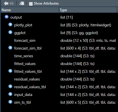
Now, let’s explore each element.

First the forecast simulation data.

output$forecast_sim

            sim_1    sim_2    sim_3    sim_4    sim_5    sim_6    sim_7
Jan 1961 445.7399 434.7175 462.6173 447.8849 453.5069 443.0944 464.4749
Feb 1961 424.1606 423.3814 431.9512 420.4460 426.8245 423.4784 443.1545
Mar 1961 444.0015 467.6276 459.3452 450.2936 453.6116 461.3751 462.4351
Apr 1961 490.2370 504.9129 492.0632 491.2198 494.6883 489.6674 498.7902
May 1961 502.0907 517.7794 504.5420 503.7614 504.8544 504.1816 521.9044
Jun 1961 552.6359 588.4650 560.1199 567.5266 563.5353 552.8411 543.5723
Jul 1961 655.1872 666.8450 642.9804 653.4262 646.1559 648.1923 639.6587
Aug 1961 633.4657 635.5080 644.1405 650.1333 631.2688 630.4410 623.3784
Sep 1961 536.3259 551.6068 548.9176 554.8289 533.3672 553.5334 529.2182
Oct 1961 486.2815 513.2851 514.8842 513.2190 481.4636 495.1295 490.7402
Nov 1961 406.9061 428.0550 437.2211 435.3443 426.4892 425.9885 416.1940
Dec 1961 454.1048 478.1804 477.3923 475.0052 504.0761 486.3584 472.2933
            sim_8    sim_9   sim_10   sim_11   sim_12   sim_13   sim_14
Jan 1961 444.3152 444.3203 453.5722 438.0253 438.0253 425.2956 458.6829
Feb 1961 418.1653 418.2569 423.9229 413.1814 404.0688 403.3318 445.9250
Mar 1961 450.8166 437.2694 452.5463 433.7963 450.5365 433.6445 448.2279
Apr 1961 489.4801 501.5545 504.4428 488.2243 503.9232 476.7711 495.1634
May 1961 499.7523 499.2059 508.6748 496.3915 520.8837 489.1480 502.1013
Jun 1961 562.7791 574.2660 571.6261 560.3126 578.8797 564.5855 581.8097
Jul 1961 653.2719 655.1924 655.0359 647.2704 664.1505 660.7023 654.6549
Aug 1961 649.6533 639.4611 655.1187 610.5014 661.2034 606.4399 654.0751
Sep 1961 542.5110 548.6498 560.1903 505.3303 552.4413 515.2890 547.9581
Oct 1961 505.5032 490.4686 495.1026 464.1546 503.7735 479.0465 501.3405
Nov 1961 423.0761 414.9520 445.9182 399.1634 435.6692 405.7617 447.0409
Dec 1961 454.4311 452.3740 473.5319 435.0425 468.3699 449.6422 474.2666
           sim_15   sim_16   sim_17   sim_18   sim_19   sim_20   sim_21
Jan 1961 455.4787 451.0585 459.4839 444.3242 435.1001 443.7523 444.9274
Feb 1961 439.4881 422.0447 442.7488 427.5273 412.6110 430.0844 418.5412
Mar 1961 473.0626 449.9922 479.0381 454.4156 443.6824 454.0246 455.8716
Apr 1961 497.0203 501.5911 517.4542 495.3593 476.1640 489.3426 492.7721
May 1961 515.2215 526.5615 506.5715 487.1920 504.6323 500.4116 506.1908
Jun 1961 576.5544 581.4492 560.9466 560.1496 557.4915 551.0780 580.6906
Jul 1961 662.4222 675.8571 643.9878 645.8877 634.9354 649.0339 655.5332
Aug 1961 648.2923 653.8785 639.1892 624.4315 643.3871 630.6072 638.5270
Sep 1961 548.8370 547.7029 548.0178 529.7305 552.4617 533.3734 541.2910
Oct 1961 500.8130 500.6410 509.7552 481.4202 500.3374 484.8628 513.4386
Nov 1961 448.3088 427.7597 434.1320 424.8617 468.9838 421.0139 460.0366
Dec 1961 479.2161 468.6392 473.0734 460.6548 492.5949 445.3285 483.7701
           sim_22   sim_23   sim_24   sim_25   sim_26   sim_27   sim_28
Jan 1961 431.9061 436.9803 445.6030 470.3241 438.1303 438.0355 442.8814
Feb 1961 405.5096 406.4255 431.2780 451.1454 438.4957 414.3992 406.9653
Mar 1961 437.8384 437.3900 455.2998 472.2864 457.3227 452.7172 439.0830
Apr 1961 480.2212 479.1317 491.4019 520.8334 492.1962 497.7494 495.6963
May 1961 507.5101 491.4699 502.3217 522.6236 504.1139 498.8398 490.4093
Jun 1961 565.3556 555.2957 562.9435 569.6062 575.3107 565.8427 558.4052
Jul 1961 631.8589 643.0705 649.3241 656.5773 699.1111 660.5835 656.7441
Aug 1961 636.9621 620.3416 635.3089 658.5513 666.7588 655.0455 634.5556
Sep 1961 533.4397 546.0061 537.0957 552.6849 578.5525 563.2023 557.6656
Oct 1961 493.0531 483.6816 489.7577 517.3445 535.8427 509.2783 506.7000
Nov 1961 421.6430 429.6623 419.7854 427.1834 456.2713 429.0018 434.0667
Dec 1961 452.2728 457.5337 460.9375 470.2428 514.2062 482.2928 490.3966
           sim_29   sim_30   sim_31   sim_32   sim_33   sim_34   sim_35
Jan 1961 455.3775 444.3272 461.2236 433.8962 464.4749 438.0355 439.1887
Feb 1961 426.9441 418.2812 447.4852 424.0317 409.7277 415.1395 433.4188
Mar 1961 457.7136 440.5773 468.7090 447.5754 438.9636 443.0306 420.3961
Apr 1961 505.5824 483.8879 508.5020 490.2527 475.6410 497.7693 480.1376
May 1961 502.1128 495.2827 526.9527 488.3082 510.2163 524.8456 504.3970
Jun 1961 564.2560 565.1836 571.4699 554.6782 548.1972 582.0468 557.3177
Jul 1961 675.1975 656.7991 674.3476 643.9736 631.1844 665.9546 650.1157
Aug 1961 642.3301 604.3293 649.4941 612.8896 632.0786 640.5119 626.3405
Sep 1961 546.0228 520.2840 550.9040 533.3240 544.4996 540.7844 555.0268
Oct 1961 517.2212 480.8524 494.4332 467.0373 505.1177 495.0939 511.8599
Nov 1961 436.9353 409.0263 423.5813 407.0598 433.9868 420.4208 435.3652
Dec 1961 477.7085 444.2295 463.2785 447.8678 471.4819 477.0888 486.3902
           sim_36   sim_37   sim_38   sim_39   sim_40   sim_41   sim_42
Jan 1961 458.2243 453.5069 442.9633 437.7823 456.7181 439.1887 444.2746
Feb 1961 437.0087 430.5385 443.4436 434.5281 441.0503 415.1167 410.6375
Mar 1961 450.4477 456.5806 462.1142 454.3194 453.8004 433.9958 450.8734
Apr 1961 507.2234 499.3962 524.0761 495.3350 498.6223 465.6067 489.4286
May 1961 521.1416 518.5159 541.6983 514.5651 504.7369 474.7817 504.5533
Jun 1961 579.8129 580.3206 598.3710 558.8196 564.7209 544.2263 569.3150
Jul 1961 685.2838 663.2947 685.4005 652.3353 664.4497 622.2188 654.6807
Aug 1961 671.5436 671.9516 655.8918 630.8036 628.7970 615.9232 637.1259
Sep 1961 566.4307 567.5127 576.3038 539.0021 523.1752 530.4702 525.4079
Oct 1961 506.4949 510.5275 513.7364 488.4346 483.6546 479.5688 482.5080
Nov 1961 455.9362 453.4418 460.7156 417.2549 413.5535 408.8823 397.0385
Dec 1961 487.4205 481.4040 488.4877 455.6214 481.9331 453.4355 448.3142
           sim_43   sim_44   sim_45   sim_46   sim_47   sim_48   sim_49
Jan 1961 456.7181 448.9127 444.1944 439.1887 444.3762 443.9540 449.6957
Feb 1961 415.5481 417.4993 432.0998 418.8621 411.7694 419.4677 432.5796
Mar 1961 441.1190 446.8376 453.2327 448.5254 448.2663 470.9662 455.3371
Apr 1961 484.0184 474.0491 510.7521 487.2088 508.1952 505.5636 510.9074
May 1961 474.5845 493.5429 520.5754 493.9236 521.0746 494.3940 527.4129
Jun 1961 540.3995 553.2761 571.1053 570.3663 579.1209 553.5803 571.8349
Jul 1961 649.1646 657.5268 653.2605 657.5574 676.0876 607.8539 654.0949
Aug 1961 643.3467 635.9533 636.3980 656.9203 673.6242 590.6108 632.1774
Sep 1961 539.6460 532.2568 541.7711 546.2181 564.7882 492.5588 501.7329
Oct 1961 490.9799 483.5566 507.1510 500.1024 505.8764 471.2807 448.5220
Nov 1961 412.2859 415.6316 428.0756 413.5517 434.7768 384.6290 382.9796
Dec 1961 461.1189 422.9218 457.3822 459.4905 484.2661 434.8731 429.3802
           sim_50
Jan 1961 442.9633
Feb 1961 382.3990
Mar 1961 411.8363
Apr 1961 459.1659
May 1961 458.3228
Jun 1961 524.1910
Jul 1961 615.5164
Aug 1961 614.8716
Sep 1961 506.6345
Oct 1961 444.9304
Nov 1961 383.3882
Dec 1961 426.0341

output$forecast_sim_tbl

# A tibble: 600 × 4
       x     y n        id
   <dbl> <dbl> <chr> <int>
 1 1961.  446. sim_1     1
 2 1961.  424. sim_1     2
 3 1961.  444. sim_1     3
 4 1961.  490. sim_1     4
 5 1961.  502. sim_1     5
 6 1961.  553. sim_1     6
 7 1962.  655. sim_1     7
 8 1962.  633. sim_1     8
 9 1962.  536. sim_1     9
10 1962.  486. sim_1    10
# … with 590 more rows

The time series that was used.

output$time_series

     Jan Feb Mar Apr May Jun Jul Aug Sep Oct Nov Dec
1949 112 118 132 129 121 135 148 148 136 119 104 118
1950 115 126 141 135 125 149 170 170 158 133 114 140
1951 145 150 178 163 172 178 199 199 184 162 146 166
1952 171 180 193 181 183 218 230 242 209 191 172 194
1953 196 196 236 235 229 243 264 272 237 211 180 201
1954 204 188 235 227 234 264 302 293 259 229 203 229
1955 242 233 267 269 270 315 364 347 312 274 237 278
1956 284 277 317 313 318 374 413 405 355 306 271 306
1957 315 301 356 348 355 422 465 467 404 347 305 336
1958 340 318 362 348 363 435 491 505 404 359 310 337
1959 360 342 406 396 420 472 548 559 463 407 362 405
1960 417 391 419 461 472 535 622 606 508 461 390 432

The fitted values in two different formats

output$fitted_values

          Jan      Feb      Mar      Apr      May      Jun      Jul      Aug
1949 111.9353 117.9664 131.9662 128.9774 120.9892 134.9782 147.9692 147.9731
1950 115.4270 121.3807 138.5312 137.2522 127.5180 139.7865 158.9159 166.3207
1951 132.8130 151.5147 164.7662 165.5934 153.1413 186.9835 201.0564 197.1598
1952 171.2150 174.9573 205.3873 181.9983 189.5111 191.9692 229.3659 230.2887
1953 197.4932 205.0669 211.9492 214.7030 229.4790 261.9978 259.3789 272.3394
1954 205.8921 206.1940 236.4993 236.1932 227.3492 247.7618 281.4459 303.3972
1955 229.7559 221.0431 274.5806 260.1968 270.5411 299.1164 345.0987 346.2332
1956 283.9172 273.9637 307.7212 313.9008 312.5977 358.8094 415.5070 394.8641
1957 313.6903 307.2137 343.5753 347.2471 353.0923 409.4687 455.6903 452.6105
1958 346.2681 328.3116 377.2767 360.7205 361.5534 432.0632 479.8147 490.8438
1959 346.5194 335.2349 385.8185 384.9676 406.8419 485.3013 531.0698 553.0149
1960 418.4120 397.2579 454.0138 420.2105 468.2327 523.6974 603.6761 623.9211
          Sep      Oct      Nov      Dec
1949 135.9874 119.0049 104.0187 118.0778
1950 156.2023 139.1631 119.1047 128.9974
1951 185.1990 158.4085 140.6879 169.2312
1952 220.7255 190.3056 172.8446 191.9035
1953 238.8716 218.7628 194.3686 207.1910
1954 261.6971 232.5912 199.3564 222.5606
1955 309.8394 277.5670 246.5073 264.0691
1956 363.2702 318.0959 271.0990 310.9291
1957 409.6920 354.9782 312.2741 341.2514
1958 438.0323 360.3301 317.3131 346.5759
1959 454.6235 412.1130 357.5358 384.6475
1960 513.8591 450.7760 410.8955 439.9468

output$fitted_values_tbl

# A tibble: 144 × 2
   index     value
   <yearmon> <dbl>
 1 Jan 1949   112.
 2 Feb 1949   118.
 3 Mar 1949   132.
 4 Apr 1949   129.
 5 May 1949   121.
 6 Jun 1949   135.
 7 Jul 1949   148.
 8 Aug 1949   148.
 9 Sep 1949   136.
10 Oct 1949   119.
# … with 134 more rows

The residual values in two different formats

output$residual_values

               Jan           Feb           Mar           Apr           May
1949   0.064663218   0.033565844   0.033806149   0.022551853   0.010753877
1950  -0.426993657   4.619296276   2.468817592  -2.252222539  -2.517970381
1951  12.187004737  -1.514734464  13.233788623  -2.593406722  18.858703025
1952  -0.215049450   5.042657391 -12.387298452  -0.998279160  -6.511066526
1953  -1.493243603  -9.066863638  24.050789583  20.296981218  -0.479038408
1954  -1.892145409 -18.194023466  -1.499295070  -9.193240870   6.650775967
1955  12.244087324  11.956865808  -7.580632008   8.803192574  -0.541058565
1956   0.082775370   3.036286487   9.278782426  -0.900756132   5.402300489
1957   1.309660582  -6.213658164  12.424731881   0.752860797   1.907693986
1958  -6.268081829 -10.311568418 -15.276674427 -12.720532082   1.446551672
1959  13.480639348   6.765147100  20.181485627  11.032373098  13.158068772
1960  -1.412019863  -6.257914445 -35.013829003  40.789527421   3.767286916
               Jun           Jul           Aug           Sep           Oct
1949   0.021825883   0.030792890   0.026927580   0.012574909  -0.004856125
1950   9.213518228  11.084130208   3.679258769   1.797714396  -6.163078961
1951  -8.983477860  -2.056432959   1.840247841  -1.199018264   3.591516610
1952  26.030752750   0.634055619  11.711292178 -11.725472510   0.694363698
1953 -18.997830355   4.621111100  -0.339432546  -1.871647726  -7.762821892
1954  16.238163730  20.554095186 -10.397216564  -2.697121208  -3.591173672
1955  15.883576851  18.901348128   0.766758698   2.160561460  -3.567021842
1956  15.190550278  -2.507027255  10.135908860  -8.270245332 -12.095862166
1957  12.531339373   9.309735715  14.389487605  -5.692026179  -7.978198549
1958   2.936791273  11.185298228  14.156225803 -34.032306461  -1.330101426
1959 -13.301336524  16.930226311   5.985059029   8.376509562  -5.112953069
1960  11.302583143  18.323916561 -17.921058274  -5.859106651  10.223989361
               Nov           Dec
1949  -0.018746667  -0.077775679
1950  -5.104668785  11.002554045
1951   5.312079856  -3.231170377
1952  -0.844622054   2.096450492
1953 -14.368618246  -6.190983141
1954   3.643587684   6.439397882
1955  -9.507327199  13.930943896
1956  -0.099013624  -4.929146809
1957  -7.274091927  -5.251369244
1958  -7.313133943  -9.575869505
1959   4.464243872  20.352533059
1960 -20.895479201  -7.946822359

output$residual_values_tbl

# A tibble: 144 × 2
   index        value
   <yearmon>    <dbl>
 1 Jan 1949   0.0647 
 2 Feb 1949   0.0336 
 3 Mar 1949   0.0338 
 4 Apr 1949   0.0226 
 5 May 1949   0.0108 
 6 Jun 1949   0.0218 
 7 Jul 1949   0.0308 
 8 Aug 1949   0.0269 
 9 Sep 1949   0.0126 
10 Oct 1949  -0.00486
# … with 134 more rows

The input data itself

output$input_data

# A tibble: 144 × 2
   index     value
   <yearmon> <dbl>
 1 Jan 1949    112
 2 Feb 1949    118
 3 Mar 1949    132
 4 Apr 1949    129
 5 May 1949    121
 6 Jun 1949    135
 7 Jul 1949    148
 8 Aug 1949    148
 9 Sep 1949    136
10 Oct 1949    119
# … with 134 more rows

The time series simulations

output$sim_ts_tbl

# A tibble: 600 × 5
   index         x     y n        id
   <yearmon> <dbl> <dbl> <chr> <int>
 1 Jan 1961  1961.  446. sim_1     1
 2 Feb 1961  1961.  424. sim_1     2
 3 Mar 1961  1961.  444. sim_1     3
 4 Apr 1961  1961.  490. sim_1     4
 5 May 1961  1961.  502. sim_1     5
 6 Jun 1961  1961.  553. sim_1     6
 7 Jul 1961  1962.  655. sim_1     7
 8 Aug 1961  1962.  633. sim_1     8
 9 Sep 1961  1962.  536. sim_1     9
10 Oct 1961  1962.  486. sim_1    10
# … with 590 more rows

Now, the visuals, first the static ggplot

output$ggplot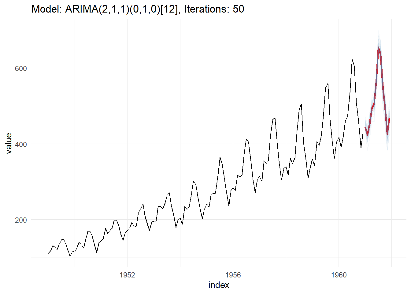

The interactive plotly plot.

output$plotly_plot

Voila!