Introduction

Are you looking for a powerful and efficient library for time series analysis? Look no further than {healthyR.ts}! This library has recently been updated with new functions and improvements, making it easier for you to analyze and visualize your time series data.

One of the new functions in {healthyR.ts} is ts_geometric_brownian_motion(). This function allows you to generate multiple Brownian motion simulations at once, saving you time and effort. With this feature, you can easily generate multiple simulations to compare and analyze different scenarios.

Another new function, ts_brownian_motion_augment(), enables you to add a Brownian motion to a time series that you provide. This is a great tool for analyzing the impact of random variations on your data.

The ts_geometric_brownian_motion_augment() function generates a geometric Brownian motion, allowing you to study the effects of compounding growth or decay in your time series data. And, with the ts_brownian_motion_plot() function, you can easily plot both augmented and non-augmented Brownian motion plots, giving you a visual representation of your data.

In addition to the new functions, {healthyR.ts} has also made several minor fixes and improvements. For example, the ts_brownian_motion() function has been updated and optimized, resulting in a 49x speedup due to vectorization. Additionally, all Brownian motion functions now have an attribute of .motion_type, making it easier to track and identify your data.

With all of these new features and improvements, {healthyR.ts} is the ideal library for anyone looking to analyze and visualize time series data. So, if you want to take your time series analysis to the next level, install {healthyR.ts} today!

Function

Let’s take a look at the new functions.

ts_geometric_brownian_motion(
  .num_sims = 100,
  .time = 25,
  .mean = 0,
  .sigma = 0.1,
  .initial_value = 100,
  .delta_time = 1/365,
  .return_tibble = TRUE
)

Its arguments.

.num_sims - Total number of simulations.
.time - Total time of the simulation.
.mean - Expected return
.sigma - Volatility
.initial_value - Integer representing the initial value.
.delta_time - Time step size.
.return_tibble - The default is TRUE. If set to FALSE then an object of class matrix will be returned.

ts_brownian_motion_augment(
  .data,
  .date_col,
  .value_col,
  .time = 100,
  .num_sims = 10,
  .delta_time = NULL
)

Its arguments.

.data - The data.frame/tibble being augmented.
.date_col - The column that holds the date.
.value_col - The value that is going to get augmented. The last value of this column becomes the initial value internally.
.time - How many time steps ahead.
.num_sims - How many simulations should be run.
.delta_time - Time step size.

ts_geometric_brownian_motion_augment(
  .data,
  .date_col,
  .value_col,
  .num_sims = 10,
  .time = 25,
  .mean = 0,
  .sigma = 0.1,
  .delta_time = 1/365
)

Its arguments.

.data - The data you are going to pass to the function to augment.
.date_col - The column that holds the date
.value_col - The column that holds the value
.num_sims - Total number of simulations.
.time - Total time of the simulation.
.mean - Expected return
.sigma - Volatility
.delta_time - Time step size.

ts_brownian_motion_plot(
  .data, 
  .date_col, 
  .value_col, 
  .interactive = FALSE
)

Its arguments.

.data - The data you are going to pass to the function to augment.
.date_col - The column that holds the date
.value_col - The column that holds the value
.interactive - The default is FALSE, TRUE will produce an interactive plotly plot.

Examples

First make sure you install {healthyR.ts} if you do not yet already have it, otherwise update it to gain th enew functionality.

install.packages("healthyR.ts")

Now let’s take a look at ts_geometric_brownian_motion().

library(healthyR.ts)

ts_geometric_brownian_motion()

# A tibble: 2,600 × 3
   sim_number        t     y
   <fct>         <int> <dbl>
 1 sim_number 1      1   100
 2 sim_number 2      1   100
 3 sim_number 3      1   100
 4 sim_number 4      1   100
 5 sim_number 5      1   100
 6 sim_number 6      1   100
 7 sim_number 7      1   100
 8 sim_number 8      1   100
 9 sim_number 9      1   100
10 sim_number 10     1   100
# … with 2,590 more rows

Now let’s take a look at ts_brownian_motion_augment().

rn <- rnorm(31)
df <- data.frame(
date_col = seq.Date(from = as.Date("2022-01-01"),
                      to = as.Date("2022-01-31"),
                      by = "day"),
 value = rn
)

ts_brownian_motion_augment(
  .data = df,
  .date_col = date_col,
  .value_col = value
)

# A tibble: 1,041 × 3
   sim_number  date_col    value
   <fct>       <date>      <dbl>
 1 actual_data 2022-01-01 -0.303
 2 actual_data 2022-01-02 -1.17 
 3 actual_data 2022-01-03 -1.44 
 4 actual_data 2022-01-04 -0.682
 5 actual_data 2022-01-05 -2.31 
 6 actual_data 2022-01-06 -1.19 
 7 actual_data 2022-01-07 -0.454
 8 actual_data 2022-01-08 -1.83 
 9 actual_data 2022-01-09  0.659
10 actual_data 2022-01-10 -0.150
# … with 1,031 more rows

Now ts_geometric_brownian_motion_augment().

rn <- rnorm(31)
df <- data.frame(
date_col = seq.Date(from = as.Date("2022-01-01"),
                      to = as.Date("2022-01-31"),
                      by = "day"),
 value = rn
)

ts_geometric_brownian_motion_augment(
  .data = df,
  .date_col = date_col,
  .value_col = value
)

# A tibble: 291 × 3
   sim_number  date_col    value
   <fct>       <date>      <dbl>
 1 actual_data 2022-01-01 -1.47 
 2 actual_data 2022-01-02 -1.63 
 3 actual_data 2022-01-03  1.01 
 4 actual_data 2022-01-04  1.44 
 5 actual_data 2022-01-05 -1.05 
 6 actual_data 2022-01-06 -0.599
 7 actual_data 2022-01-07 -0.393
 8 actual_data 2022-01-08  1.06 
 9 actual_data 2022-01-09 -0.121
10 actual_data 2022-01-10 -0.349
# … with 281 more rows

Now for ts_brownian_motion_plot().

ts_geometric_brownian_motion() %>%
  ts_brownian_motion_plot(.date_col = t, .value_col = y)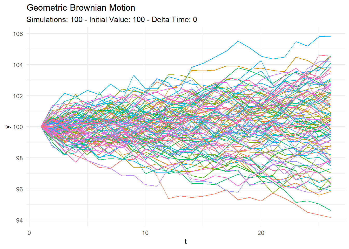

ts_brownian_motion() %>%
  ts_brownian_motion_plot(t, y, .interactive = TRUE)

And with the augmenting functions

rn <- rnorm(31)
df <- data.frame(
date_col = seq.Date(from = as.Date("2022-01-01"),
                      to = as.Date("2022-01-31"),
                      by = "day"),
 value = rn
)

ts_brownian_motion_augment(
  .data = df,
  .date_col = date_col,
  .value_col = value,
  .time = 30,
  .num_sims = 30
) %>%
  ts_brownian_motion_plot(date_col, value, TRUE)

And with a static ggplot2 plot.

rn <- rnorm(31)
df <- data.frame(
date_col = seq.Date(from = as.Date("2022-01-01"),
                      to = as.Date("2022-01-31"),
                      by = "day"),
 value = rn
)

ts_brownian_motion_augment(
  .data = df,
  .date_col = date_col,
  .value_col = value,
  .time = 30,
  .num_sims = 30
) %>%
  ts_brownian_motion_plot(date_col, value)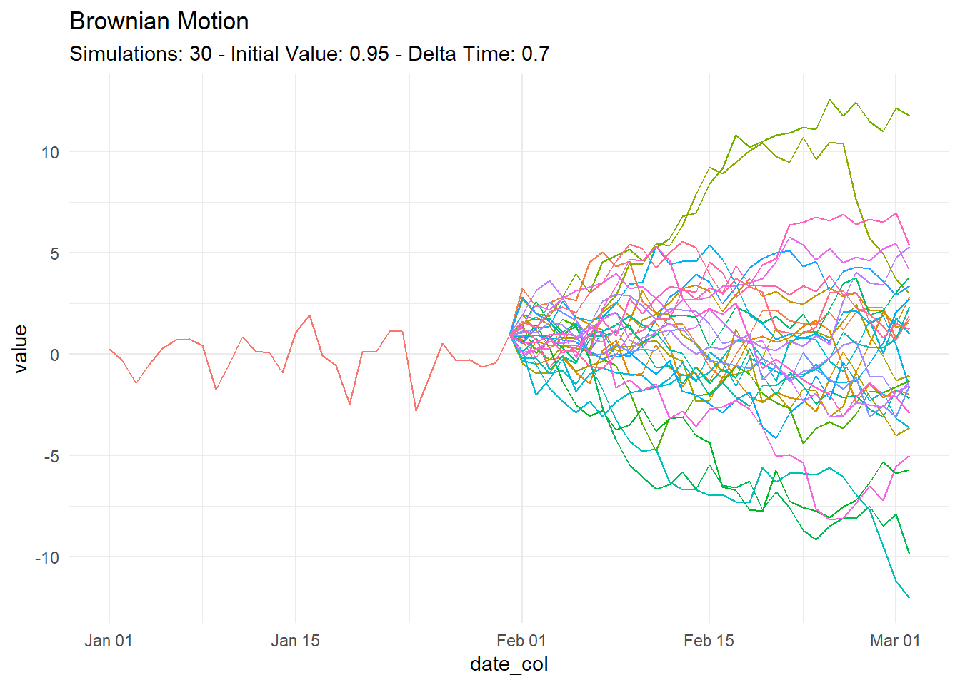

Thank you for reading, and Voila!