install.packages("healthyverse")
library(healthyverse)A Review of 2025
2025 A Year in Review
The year 2025 was a big year for me. I did a lot of coding, a lot more than I typically do. The biggest push came personally in my ongoing development of my R packages that are in the healthyverse. To use the healthyverse simply do so in the familiar fashion:
Here are links to all of the packages:
In order to start looking at some of the data that pertains to 2025 lets first get the data from the CRAN logs. Since I do this daily already, I can simply use the rds file I already have. I am going to go through the motions though, in case others might want to do something similar. The functions I am using to get the data can be found here
Now lets get that data!
library(tidyverse)
library(lubridate)
source("01_scripts/get_data_functions.R")
source("01_scripts/data_manipulation_functions.R")
source("01_scripts/mapping_functions.R")

get_cran_data()
get_package_release_data()
csv_to_rds()
Ok now that we have our data, lets ensure that we are only using the year 2025. We can do this by filtering out data by time with the timetk package.
Now lets filter our data below, some pre-processing may need to take place.
library(timetk)
data_tbl <- downloads_processed_tbl() %>%
  filter_by_time(
    .date_var = date,
    .start_date = "2025",
    .end_date = "2025"
  )

glimpse(data_tbl)
Rows: 39,070
Columns: 11
$ date <date> 2025-01-01, 2025-01-01, 2025-01-01, 2025-01-01, 2025-01-01,…
$ time <Period> 11H 41M 10S, 11H 41M 10S, 11H 41M 10S, 4H 3M 36S, 8H 26M …
$ date_time <dttm> 2025-01-01 11:41:10, 2025-01-01 11:41:10, 2025-01-01 11:41:…
$ size <int> 89711, 533, 2373526, 83942, 528, 307810, 307809, 530, 236801…
$ r_version <chr> NA, NA, NA, NA, NA, NA, NA, NA, NA, NA, NA, NA, NA, NA, "4.4…
$ r_arch <chr> NA, NA, NA, NA, NA, NA, NA, NA, NA, NA, NA, NA, NA, NA, "x86…
$ r_os <chr> NA, NA, NA, NA, NA, NA, NA, NA, NA, NA, NA, NA, NA, NA, "min…
$ package <chr> "healthyR.ts", "healthyR.ts", "healthyR.ts", "healthyverse",…
$ version <chr> "0.2.8", "0.2.8", "0.2.8", "1.0.4", "0.2.0", "0.2.0", "0.2.0…
$ country <chr> "US", "US", "US", "DE", "US", "US", "US", "US", "US", "US", …
$ ip_id <int> 684, 684, 684, 3392, 684, 684, 684, 684, 684, 684, 1394, 139…Now that we have our data, we have it for the year 2024 only with a start date of 2025-01-01 and an end date of 2025-12-31.
Package Information
The first thing we will do is look at how many downloads there were for each pacakge and it’s version.
library(knitr)

data_tbl %>%
  count(package, version) %>%
  pivot_wider(
    id_cols       = version
    , names_from  = package
    , values_from = n
    , values_fill = 0
    ) %>%
  arrange(version) %>%
kable()| version | RandomWalker | TidyDensity | healthyR | healthyR.ai | healthyR.data | healthyR.ts | healthyverse | tidyAML |
|---|---|---|---|---|---|---|---|---|
| 0.0.1 | 0 | 61 | 0 | 68 | 0 | 0 | 0 | 58 |
| 0.0.10 | 0 | 0 | 0 | 64 | 0 | 0 | 0 | 0 |
| 0.0.11 | 0 | 0 | 0 | 60 | 0 | 0 | 0 | 0 |
| 0.0.12 | 0 | 0 | 0 | 61 | 0 | 0 | 0 | 0 |
| 0.0.13 | 0 | 0 | 0 | 328 | 0 | 0 | 0 | 0 |
| 0.0.2 | 0 | 0 | 0 | 68 | 0 | 0 | 0 | 126 |
| 0.0.3 | 0 | 0 | 0 | 70 | 0 | 0 | 0 | 125 |
| 0.0.4 | 0 | 0 | 0 | 66 | 0 | 0 | 0 | 55 |
| 0.0.5 | 0 | 0 | 0 | 67 | 0 | 0 | 0 | 941 |
| 0.0.6 | 0 | 0 | 0 | 461 | 0 | 0 | 0 | 1734 |
| 0.0.7 | 0 | 0 | 0 | 67 | 0 | 0 | 0 | 0 |
| 0.0.8 | 0 | 0 | 0 | 64 | 0 | 0 | 0 | 0 |
| 0.0.9 | 0 | 0 | 0 | 71 | 0 | 0 | 0 | 0 |
| 0.1.0 | 70 | 0 | 65 | 839 | 0 | 69 | 0 | 0 |
| 0.1.1 | 0 | 0 | 57 | 2482 | 0 | 72 | 0 | 0 |
| 0.1.2 | 0 | 0 | 62 | 0 | 0 | 70 | 0 | 0 |
| 0.1.3 | 0 | 0 | 62 | 0 | 0 | 75 | 0 | 0 |
| 0.1.4 | 0 | 0 | 64 | 0 | 0 | 82 | 0 | 0 |
| 0.1.5 | 0 | 0 | 60 | 0 | 0 | 77 | 0 | 0 |
| 0.1.6 | 0 | 0 | 61 | 0 | 0 | 78 | 0 | 0 |
| 0.1.7 | 0 | 0 | 61 | 0 | 0 | 78 | 0 | 0 |
| 0.1.8 | 0 | 0 | 459 | 0 | 0 | 485 | 0 | 0 |
| 0.1.9 | 0 | 0 | 62 | 0 | 0 | 76 | 0 | 0 |
| 0.2.0 | 2422 | 0 | 63 | 0 | 0 | 77 | 0 | 0 |
| 0.2.1 | 0 | 0 | 617 | 0 | 0 | 76 | 0 | 0 |
| 0.2.10 | 0 | 0 | 0 | 0 | 0 | 75 | 0 | 0 |
| 0.2.11 | 0 | 0 | 0 | 0 | 0 | 76 | 0 | 0 |
| 0.2.2 | 0 | 0 | 2509 | 0 | 0 | 71 | 0 | 0 |
| 0.2.3 | 0 | 0 | 0 | 0 | 0 | 76 | 0 | 0 |
| 0.2.4 | 0 | 0 | 0 | 0 | 0 | 80 | 0 | 0 |
| 0.2.5 | 0 | 0 | 0 | 0 | 0 | 73 | 0 | 0 |
| 0.2.6 | 0 | 0 | 0 | 0 | 0 | 76 | 0 | 0 |
| 0.2.7 | 0 | 0 | 0 | 0 | 0 | 71 | 0 | 0 |
| 0.2.8 | 0 | 0 | 0 | 0 | 0 | 780 | 0 | 0 |
| 0.2.9 | 0 | 0 | 0 | 0 | 0 | 78 | 0 | 0 |
| 0.3.0 | 2088 | 0 | 0 | 0 | 0 | 232 | 0 | 0 |
| 0.3.1 | 0 | 0 | 0 | 0 | 0 | 2420 | 0 | 0 |
| 1.0.0 | 2239 | 51 | 0 | 0 | 85 | 0 | 79 | 0 |
| 1.0.1 | 0 | 449 | 0 | 0 | 488 | 0 | 78 | 0 |
| 1.0.2 | 0 | 0 | 0 | 0 | 406 | 0 | 156 | 0 |
| 1.0.3 | 0 | 0 | 0 | 0 | 572 | 0 | 74 | 0 |
| 1.0.4 | 0 | 0 | 0 | 0 | 0 | 0 | 336 | 0 |
| 1.1.0 | 0 | 53 | 0 | 0 | 136 | 0 | 1953 | 0 |
| 1.1.1 | 0 | 0 | 0 | 0 | 180 | 0 | 0 | 0 |
| 1.2.0 | 0 | 50 | 0 | 0 | 2132 | 0 | 0 | 0 |
| 1.2.1 | 0 | 49 | 0 | 0 | 0 | 0 | 0 | 0 |
| 1.2.2 | 0 | 48 | 0 | 0 | 0 | 0 | 0 | 0 |
| 1.2.3 | 0 | 51 | 0 | 0 | 0 | 0 | 0 | 0 |
| 1.2.4 | 0 | 472 | 0 | 0 | 0 | 0 | 0 | 0 |
| 1.2.5 | 0 | 53 | 0 | 0 | 0 | 0 | 0 | 0 |
| 1.2.6 | 0 | 125 | 0 | 0 | 0 | 0 | 0 | 0 |
| 1.3.0 | 0 | 59 | 0 | 0 | 0 | 0 | 0 | 0 |
| 1.4.0 | 0 | 50 | 0 | 0 | 0 | 0 | 0 | 0 |
| 1.5.0 | 0 | 2471 | 0 | 0 | 0 | 0 | 0 | 0 |
| 1.5.1 | 0 | 667 | 0 | 0 | 0 | 0 | 0 | 0 |
| 1.5.2 | 0 | 3367 | 0 | 0 | 0 | 0 | 0 | 0 |
Now lets see how many total downloads for the year there were for each package.
data_tbl %>%
  count(package) %>%
  set_names("Package","Total Downloads") %>%
kable()| Package | Total Downloads |
|---|---|
| RandomWalker | 6819 |
| TidyDensity | 8076 |
| healthyR | 4202 |
| healthyR.ai | 4836 |
| healthyR.data | 3999 |
| healthyR.ts | 5423 |
| healthyverse | 2676 |
| tidyAML | 3039 |
data_tbl %>%
  select(package, version) %>%
  group_by(package) %>%
  distinct() %>%
  mutate(release_count = n()) %>%
  ungroup() %>%
  select(package, release_count) %>%
  distinct() %>%
  set_names("Package", "Number of Release Downloads") %>%
kable()| Package | Number of Release Downloads |
|---|---|
| healthyR.ts | 24 |
| healthyverse | 6 |
| RandomWalker | 4 |
| TidyDensity | 16 |
| healthyR.ai | 15 |
| healthyR.data | 7 |
| healthyR | 13 |
| tidyAML | 6 |
total_number_of_releases <- data_tbl %>%
  select(package, version) %>%
  group_by(package) %>%
  distinct() %>%
  mutate(release_count = n()) %>%
  ungroup() %>%
  select(package, release_count) %>%
  distinct() %>%
  summarise(total = sum(release_count, na.rm = TRUE))
So all in all there was a total of 39,070 downloads of all the healthyverse packages in 2025. There were in total 91 package version downloads as well.
Let’s now see all the releases for the year:
pkg_rls_data_tbl <- read_csv("00_data/pkg_release_tbl.csv")

pkg_rls_data_tbl %>%
  filter_by_time(
    .date_var = date,
    .start_date = "2025",
    .end_date = "2025"
  ) %>%
  summarise(
    release_count = n(),
    .by = c(package, version)
  )
# A tibble: 7 × 3
package version release_count
<chr> <chr> <int>
1 healthyR.data 1.2.0 1
2 healthyR.ai 0.1.1 1
3 RandomWalker 0.3.0 1
4 tidyAML 0.0.6 1
5 TidyDensity 1.5.1 1
6 RandomWalker 1.0.0 1
7 TidyDensity 1.5.2 1Graphs
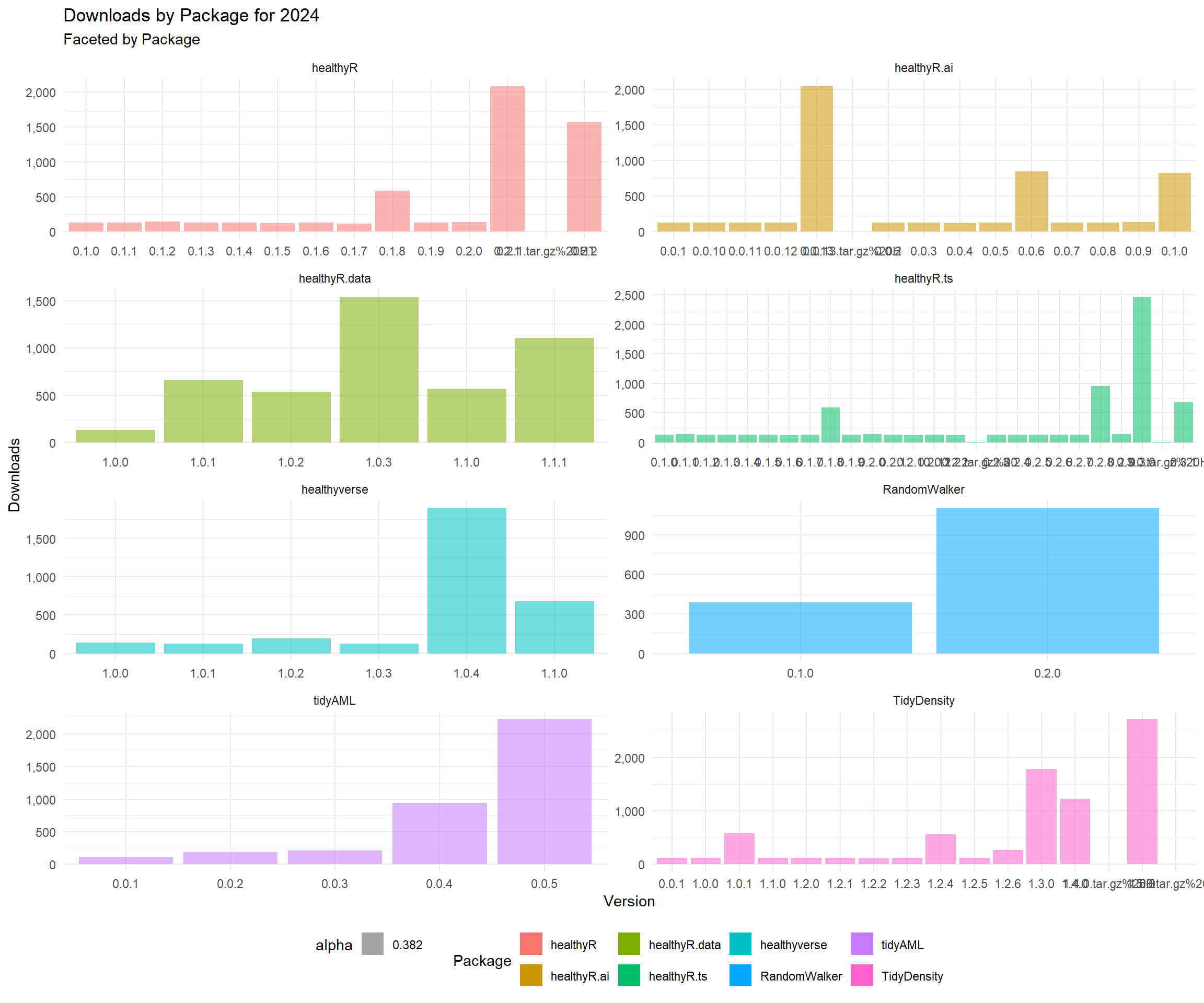
Now lets graph the data out!
data_tbl %>%
  count(package, version) %>%
  ggplot(aes(x = version, y = n, alpha = 0.382)) +
  geom_col(aes(group = package, fill = package)) +
  facet_wrap(package ~., ncol = 2, scales = "free") +
  scale_y_continuous(labels = scales::label_number(big.mark = ",")) +
  theme_minimal() +
  theme(legend.position = "bottom") +
  labs(
    title = "Downloads by Package for 2025",
    subtitle = "Faceted by Package",
    x = "Version",
    y = "Downloads",
    fill = "Package"
  )
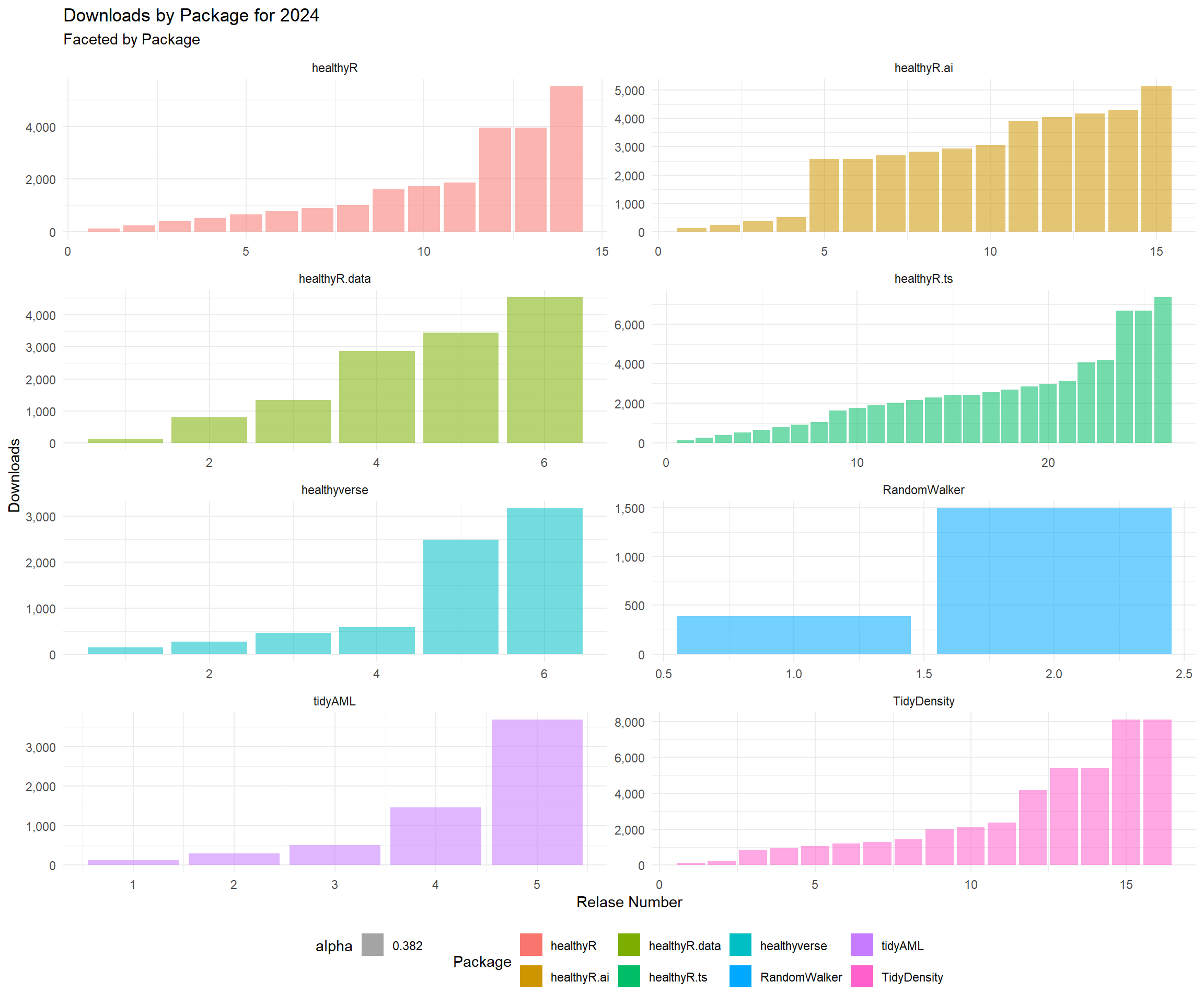
data_tbl %>%
  count(package, version) %>%
  group_by(package) %>%
  mutate(cumulative_downloads = cumsum(n)) %>%
  mutate(record = row_number()) %>%
  ungroup() %>%
  ggplot(aes(x = record, y = cumulative_downloads, alpha = 0.382)) +
  geom_col(aes(group = package, fill = package)) +
  facet_wrap(package ~., ncol = 2, scales = "free") +
  scale_y_continuous(labels = scales::label_number(big.mark = ",")) +
  theme_minimal() +
  theme(legend.position = "bottom") +
    labs(
    title = "Downloads by Package for 2025",
    subtitle = "Faceted by Package",
    x = "Relase Number",
    y = "Downloads",
    fill = "Package"
  )
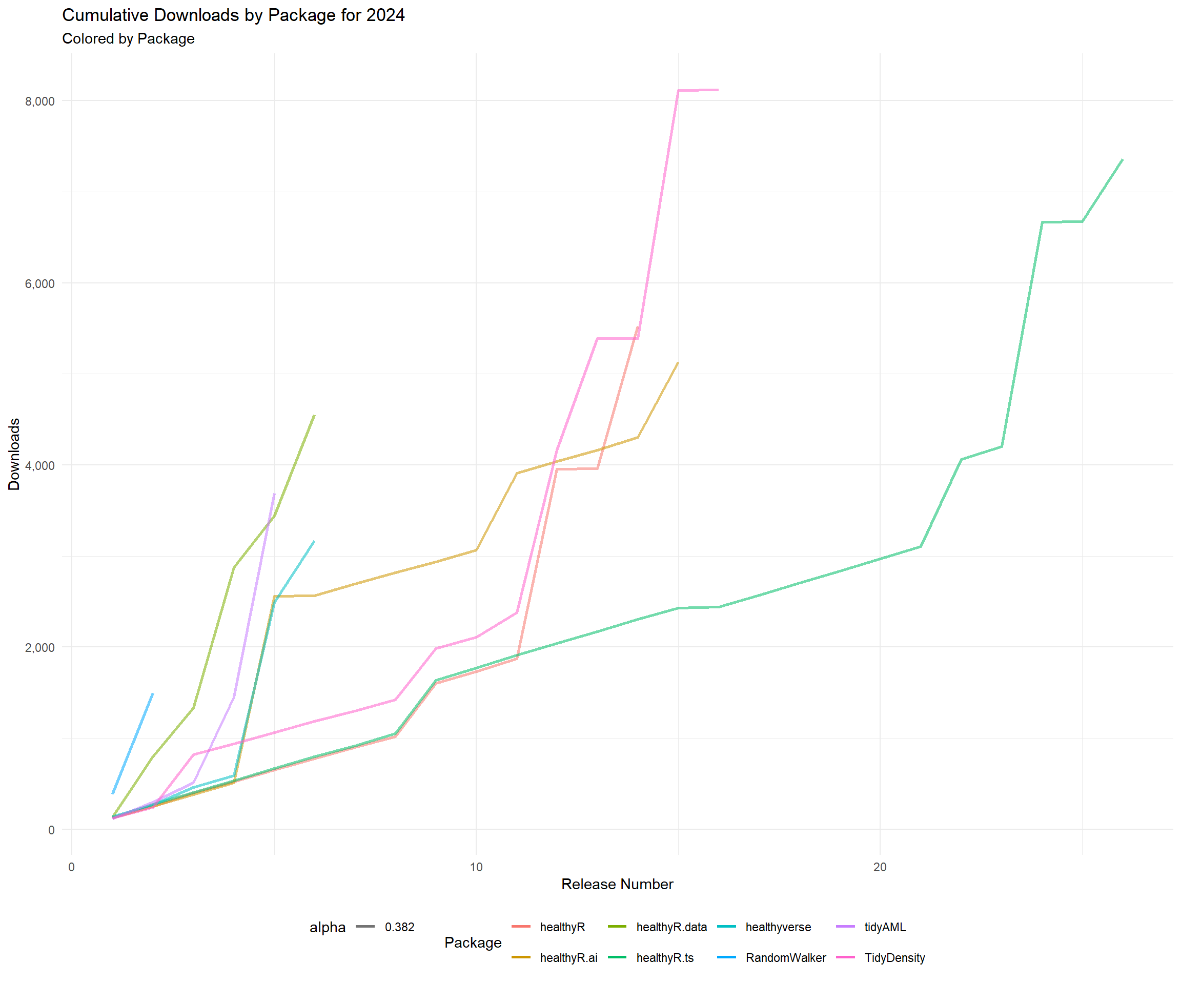
data_tbl %>%
  count(package, version) %>%
  group_by(package) %>%
  mutate(cumulative_downloads = cumsum(n)) %>%
  mutate(record = row_number()) %>%
  ungroup() %>%
  ggplot(aes(x = record, y = cumulative_downloads, alpha = 0.382)) +
  geom_line(aes(color = package, group = package), size = 1) +
  scale_y_continuous(labels = scales::label_number(big.mark = ",")) +
  theme_minimal() +
  theme(legend.position = "bottom") +
  labs(
    title = "Cumulative Downloads by Package for 2025",
    subtitle = "Colored by Package",
    x = "Release Number",
    y = "Downloads",
    color = "Package"
  )
Time Series Graphs
Now lets get some time-series graphs.
library(healthyR.ts)
pkg_tbl <- readRDS("00_data/pkg_release_tbl.rds")

data_tbl %>%
  summarise_by_time(.date_var = date, n = n()) %>%
  ts_calendar_heatmap_plot(.date_col = date, .value_col = n, .interactive = FALSE)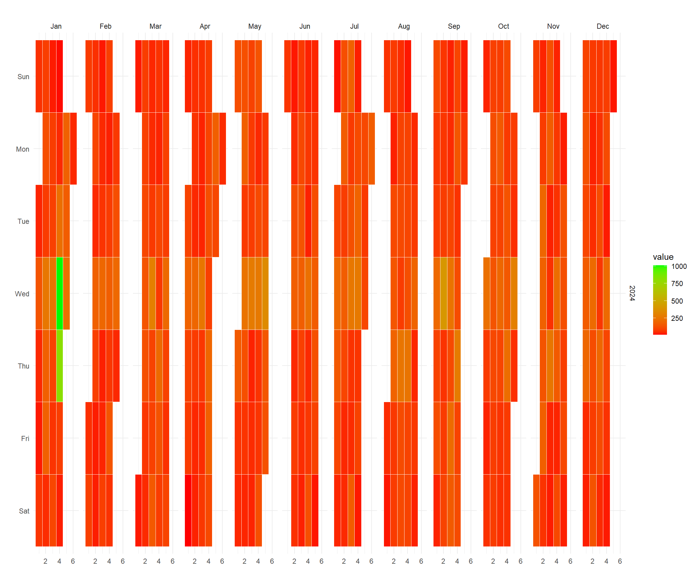
data_tbl %>%
  ts_downloads_tbl(.by_time = "day", package) %>%
  ggplot(aes(date, log1p(value))) +
  geom_point(aes(group = package, color = package), size = 1) +
  ggtitle(paste("Package Downloads: {healthyverse}")) +
  geom_smooth(method = "loess", color = "black",  se = FALSE) +
  geom_vline(
    data = pkg_tbl
    , aes(xintercept = as.Date(date))
    , color = "red"
    , lwd = 1
    , lty = "solid"
  ) +
  facet_wrap(package ~., ncol = 2, scales = "free_x") +
  theme_minimal() +
  labs(
    subtitle = "Vertical lines represent release dates",
    x = "Date",
    y = "log1p(Counts)",
    color = "Package"
  ) +
  theme(legend.position = "bottom")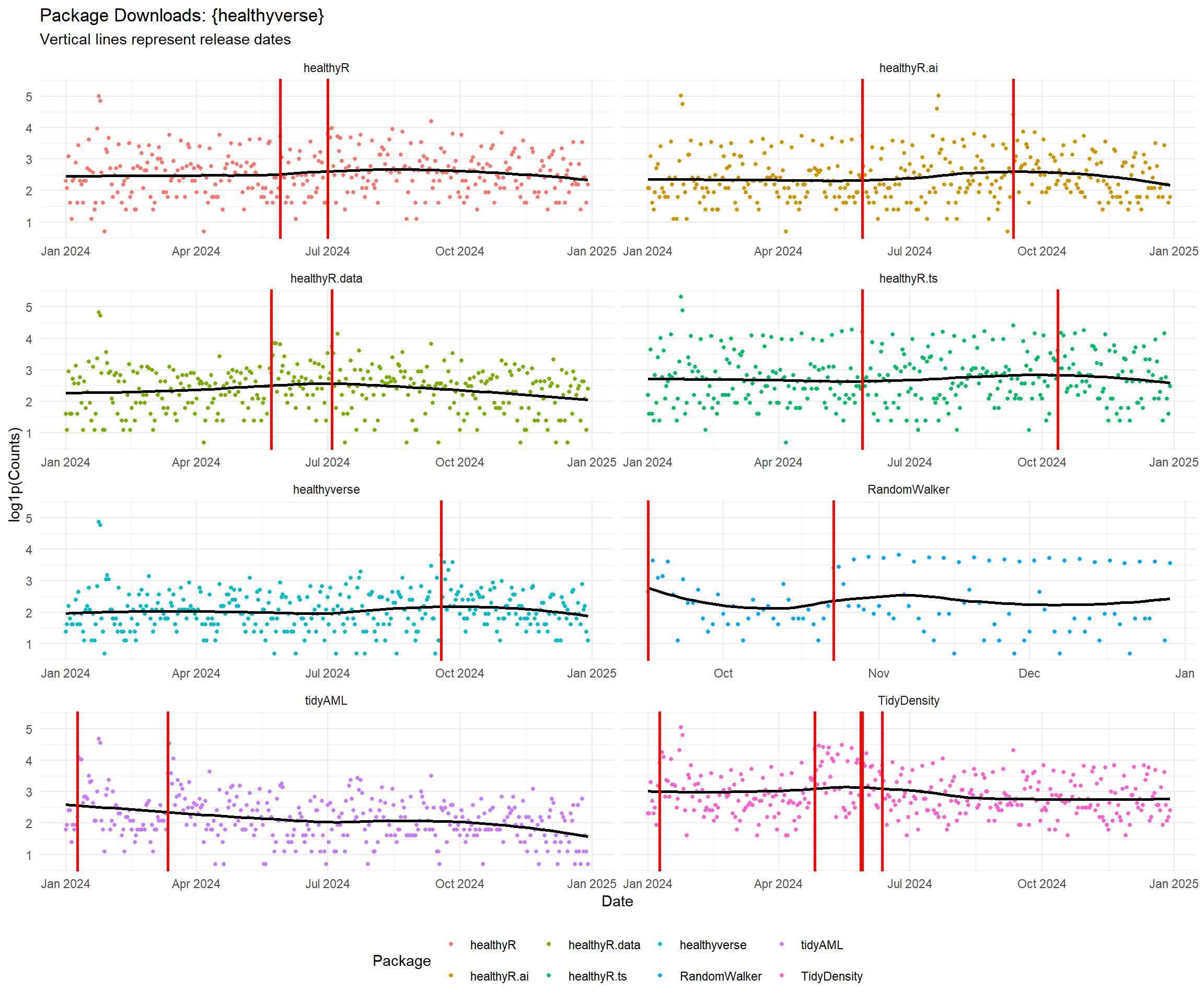
data_tbl %>%
  ts_downloads_tbl(.by_time = "day") %>%
  rename(Actual = value) %>%
  tk_augment_differences(.value = Actual, .differences = 1) %>%
  tk_augment_differences(.value = Actual, .differences = 2) %>%
  rename(velocity = contains("_diff1")) %>%
  rename(acceleration = contains("_diff2")) %>%
  pivot_longer(-date) %>%
  mutate(name = str_to_title(name)) %>%
  mutate(name = as_factor(name)) %>%
  ggplot(aes(x = date, y = log1p(value), group = name)) +
  geom_point(alpha = .2) +
  geom_vline(
    data = pkg_tbl
    , aes(xintercept = as.Date(date), color = package)
    , lwd = 1
    , lty = "solid"
  ) +
  facet_wrap(name ~ ., ncol = 1, scale = "free") +
  theme_minimal() +
  labs(
    title = "Total Downloads: Trend, Velocity, and Accelertion",
    subtitle = "Vertical Lines Indicate a CRAN Release date for a package.",
    x = "Date",
    y = "",
    color = ""
  ) +
  theme(legend.position = "bottom")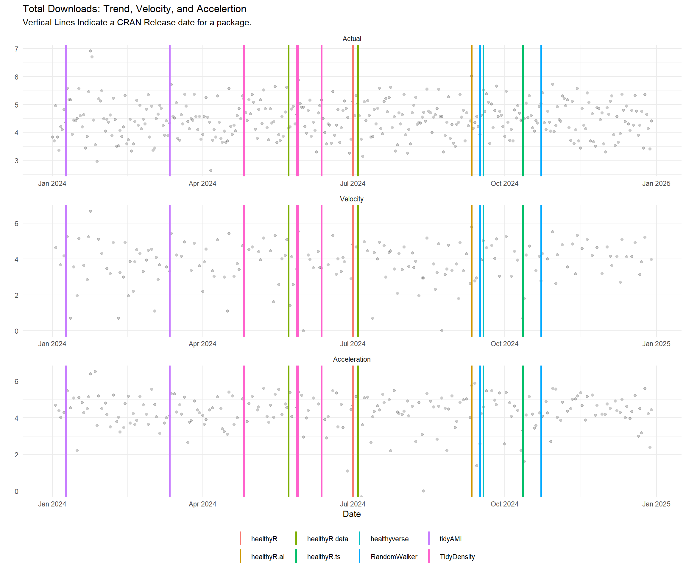
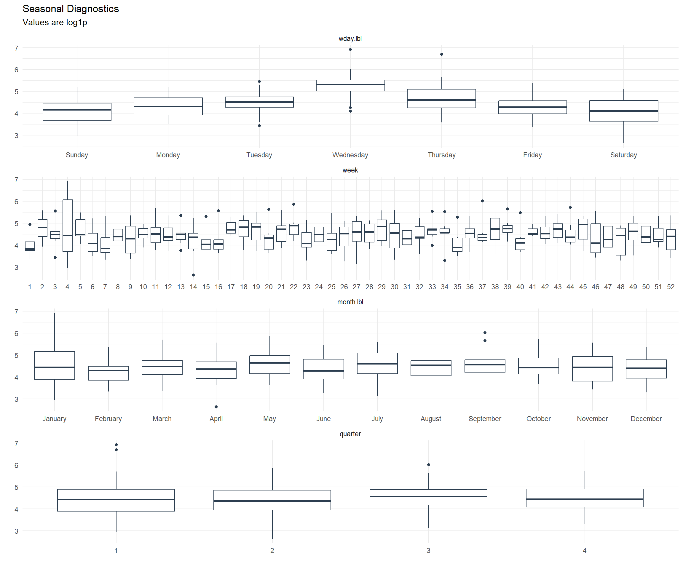
data_tbl %>%
  ts_downloads_tbl(.by_time = "day") %>%
  plot_seasonal_diagnostics(
    .date_var = date,
    .value = log1p(value),
    .interactive = FALSE
  ) +
  theme_minimal() +
  labs(
    title = "Seasonal Diagnostics",
    subtitle = "Values are log1p"
  )
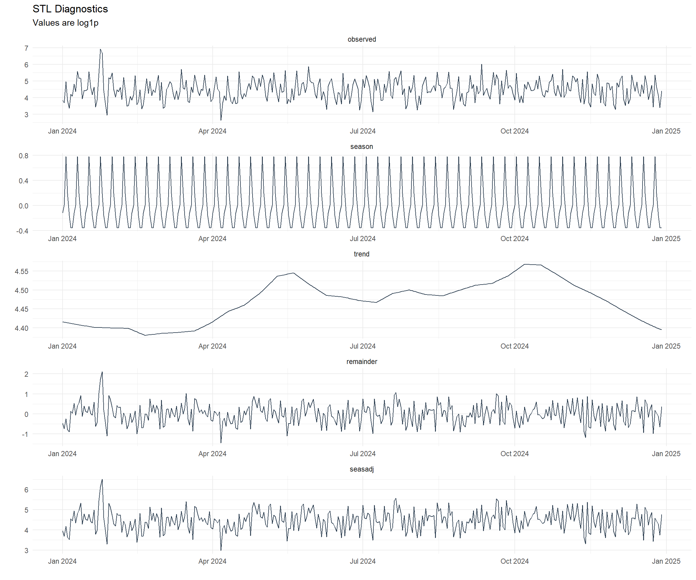
data_tbl %>%
  ts_downloads_tbl(.by_time = "day") %>%
  plot_stl_diagnostics(
    .date_var = date,
    .value = log1p(value),
    .interactive = FALSE
  ) +
  theme_minimal() +
  labs(
    title = "STL Diagnostics",
    subtitle = "Values are log1p"
  )
Mapping
So now that we have seen all the downloads in variaous ways, where did they all come from? Lets take a look.
library(tmaptools)
library(countrycode)
library(mapview)
library(htmlwidgets)
library(webshot)

# mapping_dataset(.data_year = "2025") %>%
#   head() %>%
#   knitr::kable()

l <- map_leaflet()
saveWidget(l, "downloads_map.html")
try(webshot("downloads_map.html", file = "map.png", cliprect = "viewport"))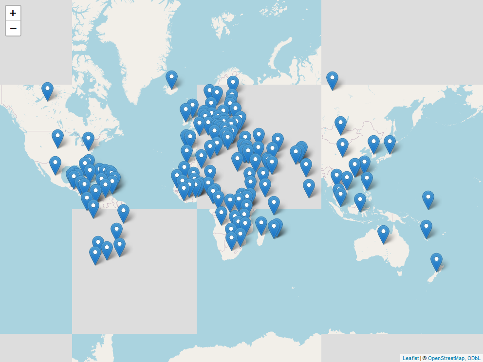
There was a total of 147 different countries that downloaded healthyverse packages in 2025.