Multi-Dimensional Walks

RandomWalker supports random walks in 1D, 2D, and 3D space. This guide covers everything you need to know about working with multi-dimensional random walks.

Overview
Generating Multi-Dimensional Walks
Understanding the Data Structure
Visualizing 2D Walks
Visualizing 3D Walks
Distance and Spatial Analysis
Use Cases
Best Practices

Overview

What are Multi-Dimensional Random Walks?

A multi-dimensional random walk extends the concept of a 1D random walk into higher-dimensional spaces:

1D: Movement along a line (left/right, up/down)
2D: Movement on a plane (x and y coordinates)
3D: Movement in space (x, y, and z coordinates)

When to Use Multi-Dimensional Walks

2D Walks: - Particle diffusion in a plane - Animal movement patterns - Robot navigation - 2D cellular automata - Currency exchange rates (two currencies vs reference)

3D Walks: - Particle diffusion in space - Molecular dynamics - Drone or aircraft movement - 3D cellular automata - Financial modeling (multiple asset classes)

Generating Multi-Dimensional Walks

Basic Syntax

All random walk generator functions support the .dimensions parameter:


# 1D walk (default)
walk_1d <- random_normal_walk(.num_walks = 5, .n = 100, .dimensions = 1)

# 2D walk
walk_2d <- random_normal_walk(.num_walks = 5, .n = 100, .dimensions = 2)

# 3D walk
walk_3d <- random_normal_walk(.num_walks = 5, .n = 100, .dimensions = 3)

All Distributions Support Multi-Dimensions

Every continuous distribution generator supports 1D, 2D, and 3D:

# 2D Brownian motion
brownian_motion(.num_walks = 10, .n = 500, .dimensions = 2)

# 3D geometric Brownian motion
geometric_brownian_motion(
  .num_walks = 10,
  .n = 500,
  .initial_value = 100,
  .dimensions = 3
)

# 2D Cauchy walk (heavy tails)
random_cauchy_walk(.num_walks = 10, .n = 200, .dimensions = 2)

# 3D exponential walk
random_exponential_walk(.num_walks = 5, .n = 300, .dimensions = 3)

Understanding the Data Structure

Column Naming Convention

1D Walk Columns:

walk_number, step_number, y, cum_sum_y, cum_prod_y, cum_min_y, cum_max_y, cum_mean_y

2D Walk Columns:

walk_number, step_number, x, y,
cum_sum_x, cum_sum_y,
cum_prod_x, cum_prod_y,
cum_min_x, cum_min_y,
cum_max_x, cum_max_y,
cum_mean_x, cum_mean_y

3D Walk Columns:

walk_number, step_number, x, y, z,
cum_sum_x, cum_sum_y, cum_sum_z,
cum_prod_x, cum_prod_y, cum_prod_z,
(and so on for each dimension)

Inspecting Multi-Dimensional Data

# 2D walk
walk_2d <- random_normal_walk(.num_walks = 3, .n = 100, .dimensions = 2)

# View structure
head(walk_2d, 10)
#> # A tibble: 10 × 14
#>    walk_number step_number       x        y cum_sum_x cum_sum_y cum_prod_x
#>    <fct>             <int>   <dbl>    <dbl>     <dbl>     <dbl>      <dbl>
#>  1 1                     1  0.0106  0.0769     0.0106    0.0769          0
#>  2 1                     2  0.133   0.153      0.143     0.230           0
#>  3 1                     3 -0.0742 -0.0912     0.0692    0.138           0
#>  4 1                     4 -0.0562 -0.00276    0.0130    0.136           0
#>  5 1                     5  0.214   0.0846     0.227     0.220           0
#>  6 1                     6  0.262   0.0412     0.489     0.261           0
#>  7 1                     7  0.0588  0.157      0.548     0.419           0
#>  8 1                     8  0.0122 -0.127      0.560     0.291           0
#>  9 1                     9 -0.0742 -0.0339     0.486     0.258           0
#> 10 1                    10  0.106  -0.0705     0.592     0.187           0
#> # ℹ 7 more variables: cum_prod_y <dbl>, cum_min_x <dbl>, cum_min_y <dbl>,
#> #   cum_max_x <dbl>, cum_max_y <dbl>, cum_mean_x <dbl>, cum_mean_y <dbl>
names(walk_2d)
#>  [1] "walk_number" "step_number" "x"           "y"           "cum_sum_x"  
#>  [6] "cum_sum_y"   "cum_prod_x"  "cum_prod_y"  "cum_min_x"   "cum_min_y"  
#> [11] "cum_max_x"   "cum_max_y"   "cum_mean_x"  "cum_mean_y"

# 3D walk
walk_3d <- random_normal_walk(.num_walks = 3, .n = 100, .dimensions = 3)

# View structure
head(walk_3d, 10)
#> # A tibble: 10 × 20
#>    walk_number step_number       x       y        z cum_sum_x cum_sum_y
#>    <fct>             <int>   <dbl>   <dbl>    <dbl>     <dbl>     <dbl>
#>  1 1                     1  0.0294 -0.0985  0.0475     0.0294   -0.0985
#>  2 1                     2 -0.222  -0.0523  0.0483    -0.193    -0.151 
#>  3 1                     3 -0.0533  0.178  -0.0974    -0.246     0.0267
#>  4 1                     4 -0.0574  0.204  -0.142     -0.304     0.231 
#>  5 1                     5  0.0642 -0.161   0.194     -0.240     0.0701
#>  6 1                     6  0.0773  0.0458  0.0483    -0.162     0.116 
#>  7 1                     7  0.0484  0.101   0.180     -0.114     0.216 
#>  8 1                     8 -0.102  -0.161  -0.00401   -0.216     0.0554
#>  9 1                     9 -0.106   0.178  -0.146     -0.322     0.233 
#> 10 1                    10 -0.120  -0.0148  0.0507    -0.442     0.218 
#> # ℹ 13 more variables: cum_sum_z <dbl>, cum_prod_x <dbl>, cum_prod_y <dbl>,
#> #   cum_prod_z <dbl>, cum_min_x <dbl>, cum_min_y <dbl>, cum_min_z <dbl>,
#> #   cum_max_x <dbl>, cum_max_y <dbl>, cum_max_z <dbl>, cum_mean_x <dbl>,
#> #   cum_mean_y <dbl>, cum_mean_z <dbl>
names(walk_3d)
#>  [1] "walk_number" "step_number" "x"           "y"           "z"          
#>  [6] "cum_sum_x"   "cum_sum_y"   "cum_sum_z"   "cum_prod_x"  "cum_prod_y" 
#> [11] "cum_prod_z"  "cum_min_x"   "cum_min_y"   "cum_min_z"   "cum_max_x"  
#> [16] "cum_max_y"   "cum_max_z"   "cum_mean_x"  "cum_mean_y"  "cum_mean_z"

Visualizing 2D Walks

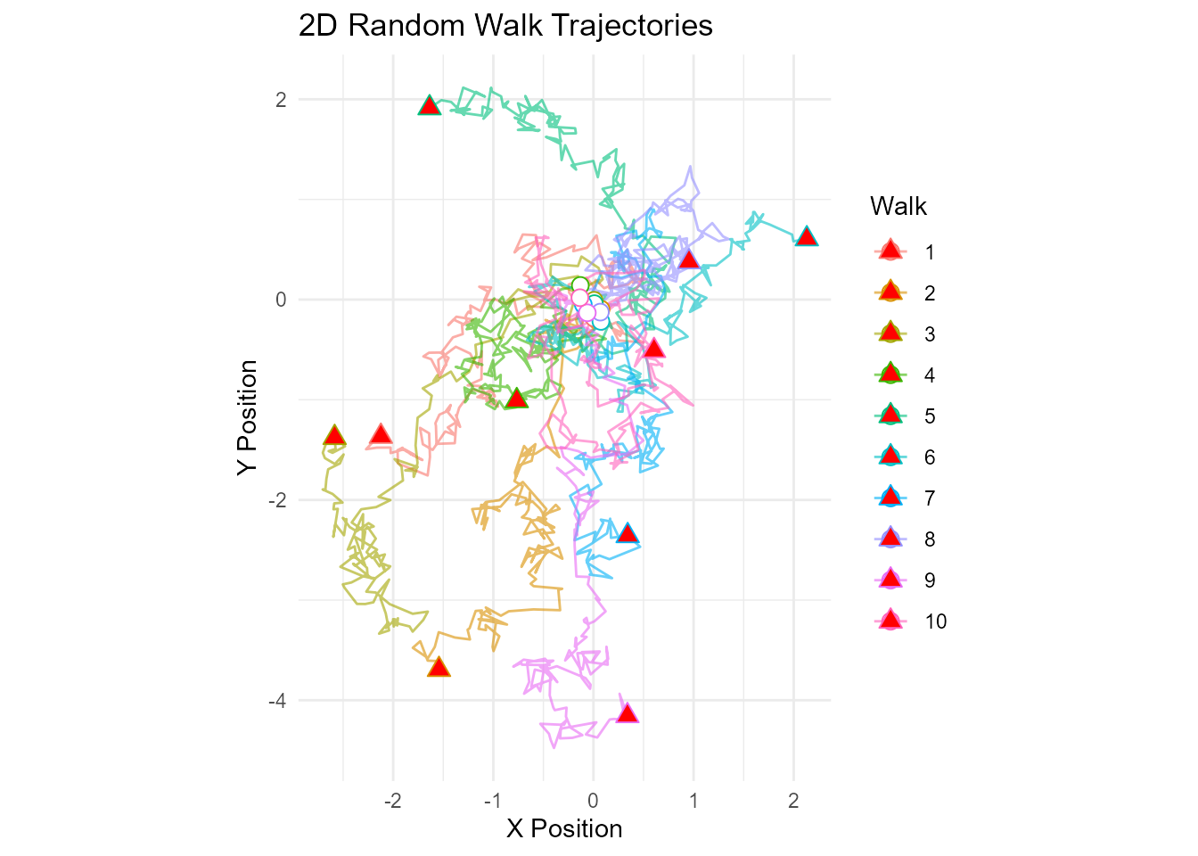
Basic 2D Trajectory Plot


# Generate 2D walk
walk_2d <- random_normal_walk(.num_walks = 10, .n = 200, .dimensions = 2)

# Plot trajectories
ggplot(walk_2d, aes(x = cum_sum_x, y = cum_sum_y, color = walk_number)) +
  geom_path(alpha = 0.6, linewidth = 0.5) +
  geom_point(data = walk_2d %>% filter(step_number == 1),
             size = 3, shape = 21, fill = "white") +  # Start points
  geom_point(data = walk_2d %>% group_by(walk_number) %>% slice_max(step_number),
             size = 3, shape = 24, fill = "red") +  # End points
  coord_equal() +
  theme_minimal() +
  labs(
    title = "2D Random Walk Trajectories",
    x = "X Position",
    y = "Y Position",
    color = "Walk"
  )

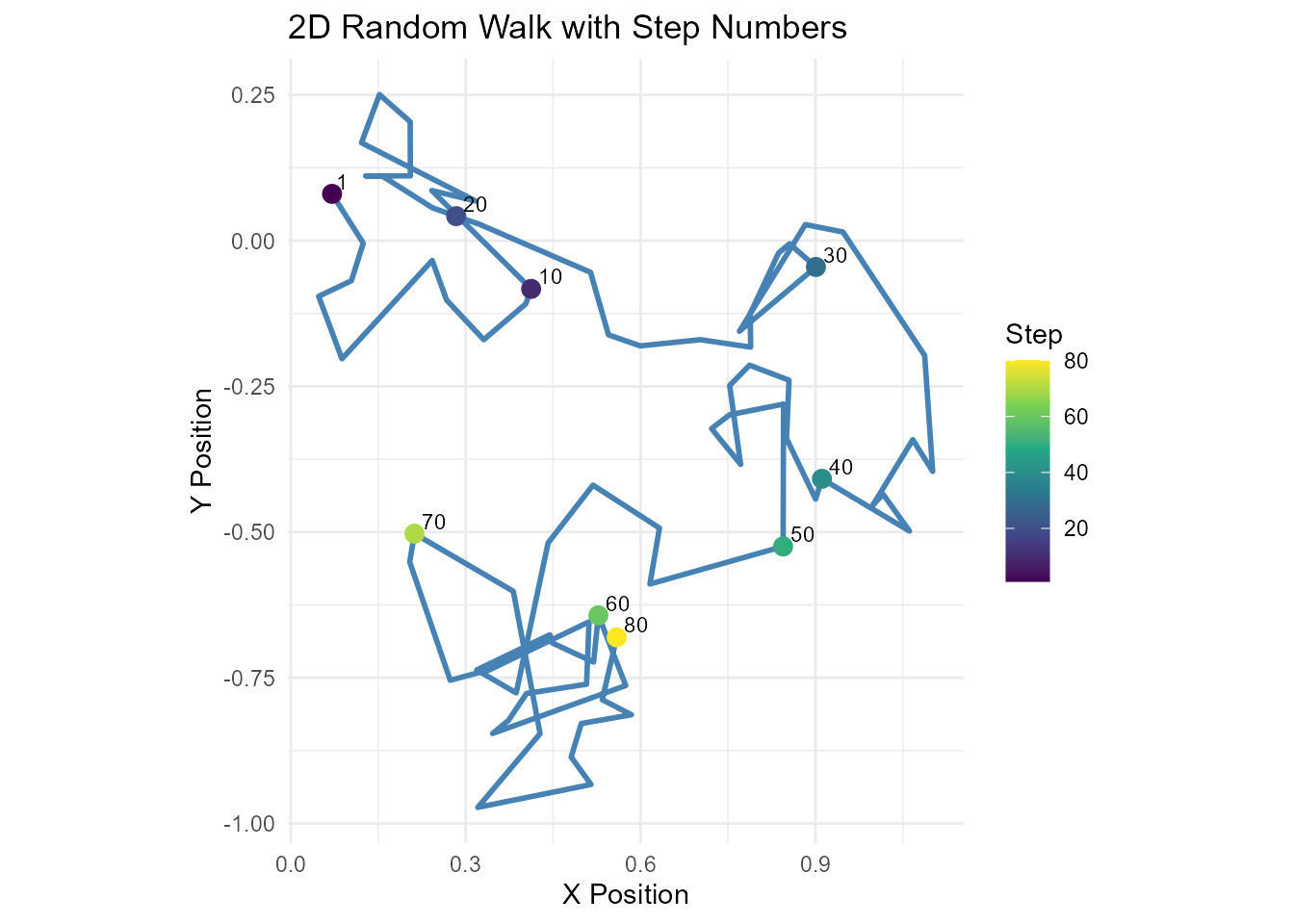
2D random walk trajectories showing multiple walks with start points marked as white circles and end points as red triangles

2D Walk with Step Numbers

# Generate single walk
walk_2d <- random_normal_walk(.num_walks = 1, .n = 100, .dimensions = 2)

# Plot with step labels at intervals
walk_2d_labeled <- walk_2d %>%
  filter(step_number %% 10 == 0 | step_number == 1)

ggplot(walk_2d, aes(x = cum_sum_x, y = cum_sum_y)) +
  geom_path(color = "steelblue", linewidth = 1) +
  geom_point(data = walk_2d_labeled, aes(color = step_number), size = 3) +
  geom_text(data = walk_2d_labeled, aes(label = step_number),
            hjust = -0.3, vjust = -0.3, size = 3) +
  scale_color_viridis_c() +
  coord_equal() +
  theme_minimal() +
  labs(
    title = "2D Random Walk with Step Numbers",
    x = "X Position",
    y = "Y Position",
    color = "Step"
  )

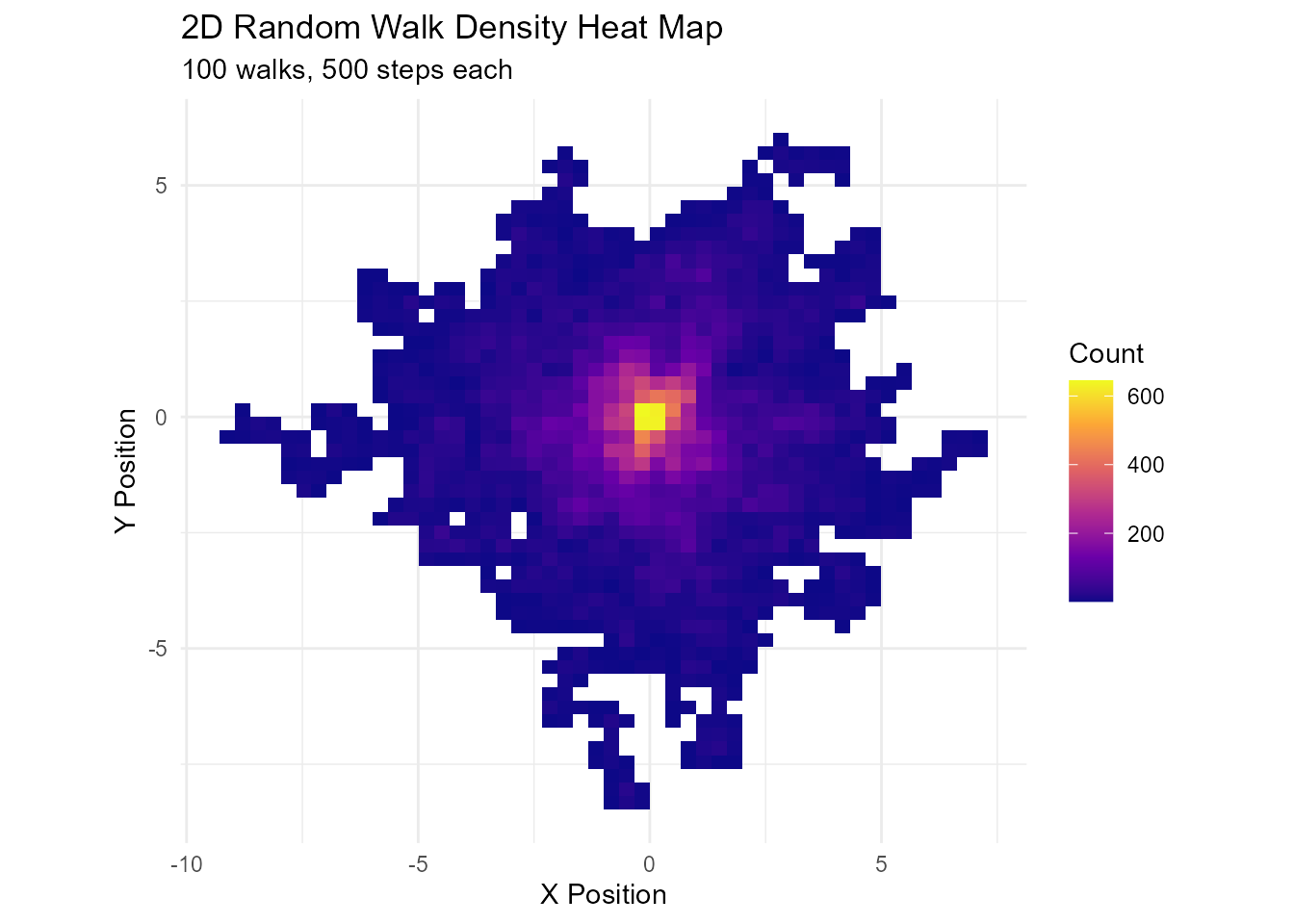
Single 2D random walk with step numbers labeled at intervals of 10 steps, colored by step progression

Heat Map of 2D Walk Density

library(ggplot2)

# Generate many walks
walk_2d <- random_normal_walk(.num_walks = 100, .n = 500, .dimensions = 2)

# Create density heat map
ggplot(walk_2d, aes(x = cum_sum_x, y = cum_sum_y)) +
  geom_bin2d(bins = 50) +
  scale_fill_viridis_c(option = "plasma") +
  coord_equal() +
  theme_minimal() +
  labs(
    title = "2D Random Walk Density Heat Map",
    subtitle = "100 walks, 500 steps each",
    x = "X Position",
    y = "Y Position",
    fill = "Count"
  )

Heat map showing the density of 100 random walks with 500 steps each, using a plasma color scale to indicate visit frequency

Animated 2D Walk

library(ggplot2)
library(gganimate)

# Generate walk
walk_2d <- random_normal_walk(.num_walks = 5, .n = 100, .dimensions = 2)

# Create animation
p <- ggplot(walk_2d, aes(x = cum_sum_x, y = cum_sum_y, color = walk_number)) +
  geom_path(aes(group = walk_number), alpha = 0.5) +
  geom_point(size = 3) +
  coord_equal() +
  theme_minimal() +
  labs(title = "Step: {frame_along}", x = "X", y = "Y") +
  transition_reveal(step_number)

# Render
animate(p, nframes = 100, fps = 10)

Visualizing 3D Walks

3D Scatter Plot

library(plotly)

# Generate 3D walk
walk_3d <- random_normal_walk(.num_walks = 5, .n = 200, .dimensions = 3)

# Create 3D plot
plot_ly(
  data = walk_3d,
  x = ~cum_sum_x,
  y = ~cum_sum_y,
  z = ~cum_sum_z,
  color = ~walk_number,
  type = "scatter3d",
  mode = "lines",
  line = list(width = 2)
) %>%
  layout(
    title = "3D Random Walk Trajectories",
    scene = list(
      xaxis = list(title = "X Position"),
      yaxis = list(title = "Y Position"),
      zaxis = list(title = "Z Position")
    )
  )

3D Interactive with Markers

library(plotly)
library(dplyr)

# Generate 3D walk
walk_3d <- random_normal_walk(.num_walks = 3, .n = 100, .dimensions = 3)

# Mark start and end points
walk_with_markers <- walk_3d %>%
  mutate(
    point_type = case_when(
      step_number == 1 ~ "Start",
      step_number == max(step_number) ~ "End",
      TRUE ~ "Path"
    )
  )

# Create plot
plot_ly(data = walk_with_markers) %>%
  # Add paths
  add_trace(
    data = walk_with_markers %>% filter(point_type == "Path"),
    x = ~cum_sum_x, y = ~cum_sum_y, z = ~cum_sum_z,
    color = ~walk_number,
    type = "scatter3d",
    mode = "lines",
    line = list(width = 2),
    showlegend = FALSE
  ) %>%
  # Add start points
  add_trace(
    data = walk_with_markers %>% filter(point_type == "Start"),
    x = ~cum_sum_x, y = ~cum_sum_y, z = ~cum_sum_z,
    type = "scatter3d",
    mode = "markers",
    marker = list(size = 8, color = "green", symbol = "circle"),
    name = "Start"
  ) %>%
  # Add end points
  add_trace(
    data = walk_with_markers %>% filter(point_type == "End"),
    x = ~cum_sum_x, y = ~cum_sum_y, z = ~cum_sum_z,
    type = "scatter3d",
    mode = "markers",
    marker = list(size = 8, color = "red", symbol = "diamond"),
    name = "End"
  ) %>%
  layout(
    title = "3D Random Walk with Start/End Markers",
    scene = list(
      xaxis = list(title = "X"),
      yaxis = list(title = "Y"),
      zaxis = list(title = "Z")
    )
  )

3D Projections

library(ggplot2)
library(patchwork)

# Generate 3D walk
walk_3d <- random_normal_walk(.num_walks = 5, .n = 200, .dimensions = 3)

# X-Y projection
p_xy <- ggplot(walk_3d, aes(x = cum_sum_x, y = cum_sum_y, color = walk_number)) +
  geom_path(alpha = 0.6) +
  coord_equal() +
  theme_minimal() +
  labs(title = "X-Y Projection")

# X-Z projection
p_xz <- ggplot(walk_3d, aes(x = cum_sum_x, y = cum_sum_z, color = walk_number)) +
  geom_path(alpha = 0.6) +
  coord_equal() +
  theme_minimal() +
  labs(title = "X-Z Projection")

# Y-Z projection
p_yz <- ggplot(walk_3d, aes(x = cum_sum_y, y = cum_sum_z, color = walk_number)) +
  geom_path(alpha = 0.6) +
  coord_equal() +
  theme_minimal() +
  labs(title = "Y-Z Projection")

# Combine
p_xy / (p_xz | p_yz) +
  plot_layout(guides = "collect") +
  plot_annotation(title = "3D Random Walk - All Projections")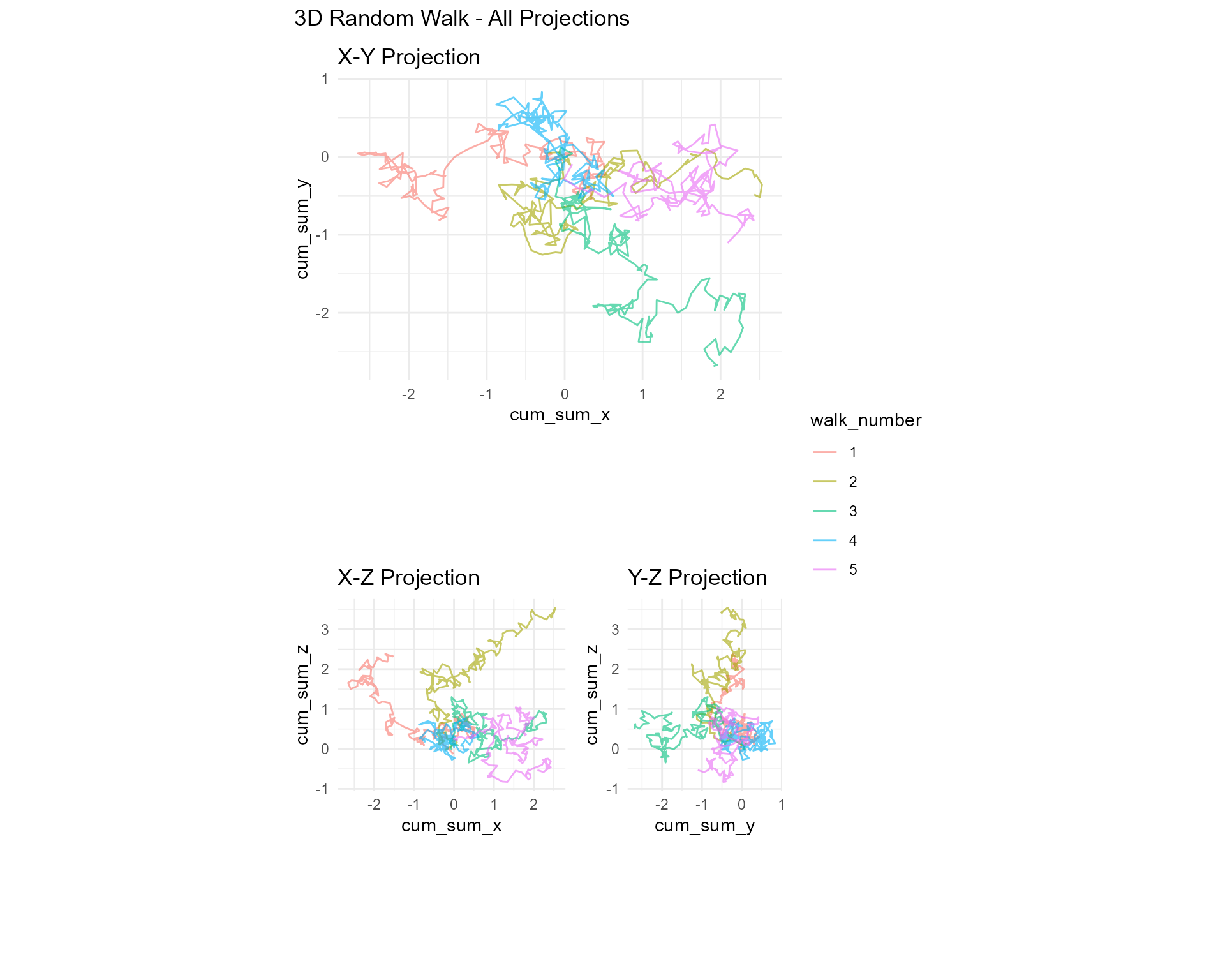

Three projection plots showing X-Y, X-Z, and Y-Z views of 3D random walks, arranged with X-Y on top and X-Z and Y-Z side by side below

Distance and Spatial Analysis

Euclidean Distance from Origin

library(dplyr)

# 2D walk
walk_2d <- random_normal_walk(.num_walks = 10, .n = 500, .dimensions = 2)

# Calculate distance
walk_with_distance <- walk_2d %>%
  euclidean_distance(.x = x, .y = y)

# Visualize distance over time
library(ggplot2)

ggplot(walk_with_distance, aes(x = step_number, y = distance, color = walk_number)) +
  geom_line(alpha = 0.7) +
  # Add theoretical expectation
  geom_line(aes(y = sqrt(2 * step_number)), color = "black", linetype = "dashed", linewidth = 1) +
  theme_minimal() +
  labs(
    title = "Distance from Origin in 2D Random Walk",
    subtitle = "Dashed line shows theoretical E[distance] = sqrt(2n)",
    x = "Step",
    y = "Euclidean Distance"
  )

3D Distance Analysis

# 3D walk
walk_3d <- random_normal_walk(.num_walks = 100, .n = 1000, .dimensions = 3)

# Calculate distance
walk_with_distance <- walk_3d %>%
  euclidean_distance(.x = x, .y = z)

# Analyze distance distribution at specific steps
library(dplyr)

distance_at_steps <- walk_with_distance %>%
  filter(step_number %in% c(100, 250, 500, 1000)) %>%
  group_by(step_number) %>%
  reframe(
    mean_dist = mean(distance),
    sd_dist = sd(distance),
    theoretical_mean = sqrt(3 * step_number)
  )

print(distance_at_steps)

Radial Distribution Function

library(dplyr)
library(ggplot2)

# Generate many 2D walks
walk_2d <- random_normal_walk(.num_walks = 500, .n = 200, .dimensions = 2)

# Get final positions
final_positions <- walk_2d %>%
  group_by(walk_number) %>%
  slice_max(step_number) %>%
  euclidean_distance(.x = x, .y = y)

# Plot radial distribution
ggplot(final_positions, aes(x = distance)) +
  geom_histogram(aes(y = after_stat(density)), bins = 50, fill = "steelblue", alpha = 0.7) +
  geom_density(color = "darkblue", linewidth = 1) +
  theme_minimal() +
  labs(
    title = "Radial Distribution of Final Positions (2D)",
    subtitle = "500 walks, 200 steps each",
    x = "Distance from Origin",
    y = "Density"
  )

Convex Hull (2D)

library(dplyr)
library(ggplot2)

# Generate 2D walks
walk_2d <- random_normal_walk(.num_walks = 20, .n = 200, .dimensions = 2)

# Get final positions
final_positions <- walk_2d %>%
  group_by(walk_number) %>%
  slice_max(step_number)

# Calculate convex hull
hull <- chull(final_positions$cum_sum_x, final_positions$cum_sum_y)
hull_points <- final_positions[c(hull, hull[1]), ]  # Close the polygon

# Plot
ggplot(walk_2d, aes(x = cum_sum_x, y = cum_sum_y, color = walk_number)) +
  geom_path(alpha = 0.3) +
  geom_point(data = final_positions, size = 3) +
  geom_polygon(data = hull_points, aes(x = cum_sum_x, y = cum_sum_y),
               fill = NA, color = "black", linewidth = 1) +
  coord_equal() +
  theme_minimal() +
  labs(
    title = "2D Random Walks with Convex Hull",
    subtitle = "Black polygon shows convex hull of final positions",
    x = "X Position",
    y = "Y Position"
  )

Use Cases

Case 1: Particle Diffusion (2D)

# Simulate particle diffusion in a petri dish
particles <- brownian_motion(
  .num_walks = 50,
  .n = 1000,
  .delta_time = 0.1,
  .dimensions = 2
)

# Visualize
particles %>%
  euclidean_distance(.x = x, .y = y) %>%
  ggplot(aes(x = step_number, y = distance, color = walk_number)) +
  geom_line(alpha = 0.3) +
  stat_summary(aes(group = 1), fun = mean, geom = "line",
               color = "red", linewidth = 1.5) +
  theme_minimal() +
  labs(
    title = "Particle Diffusion in 2D",
    subtitle = "Red line shows mean distance",
    x = "Time Step",
    y = "Distance from Origin"
  )

Case 2: Drone Flight Path (3D)

# Simulate drone wandering in 3D space
drone_path <- brownian_motion(
  .num_walks = 1,
  .n = 500,
  .delta_time = 0.5,
  .initial_value = 100,  # Start at 100m altitude
  .dimensions = 3
)

# 3D visualization
library(plotly)

plot_ly(
  data = drone_path,
  x = ~cum_sum_x,
  y = ~cum_sum_y,
  z = ~cum_sum_z,
  type = "scatter3d",
  mode = "lines+markers",
  marker = list(
    size = 2,
    color = ~step_number,
    colorscale = "Viridis",
    showscale = TRUE
  ),
  line = list(width = 2, color = "steelblue")
) %>%
  layout(
    title = "Drone Flight Path (3D Random Walk)",
    scene = list(
      xaxis = list(title = "X (meters)"),
      yaxis = list(title = "Y (meters)"),
      zaxis = list(title = "Altitude (meters)")
    )
  )

Case 3: Animal Movement (2D)

# Simulate animal foraging behavior
# Using Cauchy walk for heavy tails (occasional long jumps)
animal_movement <- random_cauchy_walk(
  .num_walks = 1,
  .n = 200,
  .scale = 1,
  .dimensions = 2
)

# Add "home" location
animal_movement <- animal_movement %>%
  mutate(
    distance_from_home = sqrt(cum_sum_x^2 + cum_sum_y^2)
  )

# Plot
ggplot(animal_movement, aes(x = cum_sum_x, y = cum_sum_y)) +
  geom_path(color = "darkgreen", linewidth = 0.8, alpha = 0.6) +
  geom_point(aes(color = distance_from_home), size = 2) +
  geom_point(x = 0, y = 0, size = 5, color = "red", shape = 17) +  # Home
  scale_color_viridis_c(option = "magma") +
  coord_equal() +
  theme_minimal() +
  labs(
    title = "Animal Foraging Path (2D Cauchy Walk)",
    subtitle = "Red triangle marks home location",
    x = "X Position",
    y = "Y Position",
    color = "Distance\nfrom Home"
  )

Best Practices

Performance Considerations

For many walks or long walks in 3D:

# Reduce number of dimensions if not needed
walk_2d <- random_normal_walk(.num_walks = 100, .n = 1000, .dimensions = 2)

# Instead of
# walk_3d <- random_normal_walk(.num_walks = 100, .n = 1000, .dimensions = 3)

For visualization:

# Sample walks or steps for large datasets
walk_large <- random_normal_walk(.num_walks = 1000, .n = 1000, .dimensions = 2)

# Sample walks
walk_sample <- walk_large %>%
  filter(walk_number %in% sample(levels(walk_number), 50))

# Or downsample steps
walk_downsample <- walk_large %>%
  filter(step_number %% 10 == 0)

Coordinate Systems

Ensure equal aspect ratios for spatial plots:

# Good - maintains true spatial relationships
ggplot(walk_2d, aes(x = cum_sum_x, y = cum_sum_y)) +
  geom_path() +
  coord_equal()  # Important!

# Bad - distorts spatial relationships
ggplot(walk_2d, aes(x = cum_sum_x, y = cum_sum_y)) +
  geom_path()  # No coord_equal()

Boundary Conditions

Implement reflecting or absorbing boundaries:

# Reflecting boundary (bounce back)
walk_2d <- random_normal_walk(.num_walks = 10, .n = 500, .dimensions = 2)

walk_bounded <- walk_2d %>%
  mutate(
    cum_sum_x = pmin(pmax(cum_sum_x, -50), 50),  # Bound between -50 and 50
    cum_sum_y = pmin(pmax(cum_sum_y, -50), 50)
  )

# Visualize
ggplot(walk_bounded, aes(x = cum_sum_x, y = cum_sum_y, color = walk_number)) +
  geom_path(alpha = 0.6) +
  geom_rect(xmin = -50, xmax = 50, ymin = -50, ymax = 50,
            fill = NA, color = "black", linewidth = 1) +
  coord_equal() +
  theme_minimal() +
  labs(title = "2D Walk with Reflecting Boundaries")

Next Steps

For more information on RandomWalker, explore these resources:

Getting Started - Introduction to random walks
Basic Concepts - Core ideas and terminology
Continuous Distribution Generators - Walks based on continuous distributions
Discrete Distribution Generators - Walks based on discrete distributions
FAQ - Frequently asked questions
API Reference - Complete function documentation Need more examples? Check out the package documentation and vignettes for additional use cases and applications!

Table of Contents