Statistical Analysis Guide

RandomWalker provides comprehensive statistical analysis capabilities for random walks. This guide covers all the tools available for analyzing and understanding your random walk data.

Summary Statistics
Cumulative Functions
Confidence Intervals
Running Quantiles
Distance Calculations
Subsetting Walks
Advanced Analysis
Statistical Tests

Summary Statistics

Basic Summary with `summarize_walks()`

The summarize_walks() function computes comprehensive statistics:

# Generate walks
walks <- random_normal_walk(.num_walks = 30, .n = 100)

# Overall summary
walks |> summarize_walks(.value = y)
#> Registered S3 method overwritten by 'quantmod':
#>   method            from
#>   as.zoo.data.frame zoo
#> Warning: There was 1 warning in `dplyr::summarize()`.
#> ℹ In argument: `geometric_mean = exp(mean(log(y)))`.
#> Caused by warning in `log()`:
#> ! NaNs produced
#> # A tibble: 1 × 16
#>   fns     fns_name   obs mean_val  median range quantile_lo quantile_hi variance
#>   <chr>   <chr>    <int>    <dbl>   <dbl> <dbl>       <dbl>       <dbl>    <dbl>
#> 1 random… Random …   100  0.00157 0.00383 0.600      -0.190       0.190  0.00935
#> # ℹ 7 more variables: sd <dbl>, min_val <dbl>, max_val <dbl>,
#> #   harmonic_mean <dbl>, geometric_mean <dbl>, skewness <dbl>, kurtosis <dbl>

# Summary by walk
walks |>
  summarize_walks(.value = y, .group_var = walk_number) |>
  head()
#> Warning: There were 30 warnings in `dplyr::summarize()`.
#> The first warning was:
#> ℹ In argument: `geometric_mean = exp(mean(log(y)))`.
#> ℹ In group 1: `walk_number = 1`.
#> Caused by warning in `log()`:
#> ! NaNs produced
#> ℹ Run `dplyr::last_dplyr_warnings()` to see the 29 remaining warnings.
#> # A tibble: 6 × 17
#>   walk_number fns              fns_name   obs mean_val  median range quantile_lo
#>   <fct>       <chr>            <chr>    <int>    <dbl>   <dbl> <dbl>       <dbl>
#> 1 1           random_normal_w… Random …   100  0.00310 0.0225  0.529      -0.244
#> 2 2           random_normal_w… Random …   100  0.0124  0.00751 0.455      -0.190
#> 3 3           random_normal_w… Random …   100  0.0218  0.0319  0.317      -0.117
#> 4 4           random_normal_w… Random …   100  0.0156  0.0344  0.512      -0.202
#> 5 5           random_normal_w… Random …   100 -0.00789 0.0165  0.374      -0.207
#> 6 6           random_normal_w… Random …   100  0.00755 0.0129  0.479      -0.192
#> # ℹ 9 more variables: quantile_hi <dbl>, variance <dbl>, sd <dbl>,
#> #   min_val <dbl>, max_val <dbl>, harmonic_mean <dbl>, geometric_mean <dbl>,
#> #   skewness <dbl>, kurtosis <dbl>

Statistics Included: - fns - Function name used to generate walks - fns_name - Formatted function name - dimensions - Number of dimensions (1, 2, or 3) - mean_val - Mean of all values - median - Median value - range - Difference between max and min - quantile_lo - Lower quantile (default 0.025) - quantile_hi - Upper quantile (default 0.975) - variance - Variance - sd - Standard deviation - min_val - Minimum value - max_val - Maximum value - harmonic_mean - Harmonic mean - geometric_mean - Geometric mean - skewness - Skewness (measure of asymmetry) - kurtosis - Kurtosis (measure of tail heaviness)

Analyzing Different Values

# Summarize cumulative sum
walks |> summarize_walks(.value = cum_sum_y)
#> Warning: There was 1 warning in `dplyr::summarize()`.
#> ℹ In argument: `geometric_mean = exp(mean(log(cum_sum_y)))`.
#> Caused by warning in `log()`:
#> ! NaNs produced
#> # A tibble: 1 × 16
#>   fns      fns_name   obs mean_val median range quantile_lo quantile_hi variance
#>   <chr>    <chr>    <int>    <dbl>  <dbl> <dbl>       <dbl>       <dbl>    <dbl>
#> 1 random_… Random …   100   0.0715 0.0761  4.98       -1.24        1.45    0.456
#> # ℹ 7 more variables: sd <dbl>, min_val <dbl>, max_val <dbl>,
#> #   harmonic_mean <dbl>, geometric_mean <dbl>, skewness <dbl>, kurtosis <dbl>

# Summarize cumulative product
geometric_brownian_motion(.num_walks = 30, .initial_value = 100) |>
  summarize_walks(.value = cum_prod_y)
#> # A tibble: 1 × 17
#>   fns             fns_name dimensions   obs mean_val  median   range quantile_lo
#>   <chr>           <chr>         <dbl> <dbl>    <dbl>   <dbl>   <dbl>       <dbl>
#> 1 geometric_brow… Geometr…          1   100  7.72e30 1.66e17 2.89e33        800.
#> # ℹ 9 more variables: quantile_hi <dbl>, variance <dbl>, sd <dbl>,
#> #   min_val <dbl>, max_val <dbl>, harmonic_mean <dbl>, geometric_mean <dbl>,
#> #   skewness <dbl>, kurtosis <dbl>

# Summarize by group
walks |>
  summarize_walks(.value = cum_sum_y, .group_var = walk_number) |>
  head()
#> Warning: There were 29 warnings in `dplyr::summarize()`.
#> The first warning was:
#> ℹ In argument: `geometric_mean = exp(mean(log(cum_sum_y)))`.
#> ℹ In group 1: `walk_number = 1`.
#> Caused by warning in `log()`:
#> ! NaNs produced
#> ℹ Run `dplyr::last_dplyr_warnings()` to see the 28 remaining warnings.
#> # A tibble: 6 × 17
#>   walk_number fns              fns_name   obs mean_val  median range quantile_lo
#>   <fct>       <chr>            <chr>    <int>    <dbl>   <dbl> <dbl>       <dbl>
#> 1 1           random_normal_w… Random …   100  -0.0272 -0.0154 0.998    -0.529  
#> 2 2           random_normal_w… Random …   100   0.283   0.212  1.41     -0.267  
#> 3 3           random_normal_w… Random …   100   1.00    1.32   1.77      0.00822
#> 4 4           random_normal_w… Random …   100   1.13    1.24   1.58      0.102  
#> 5 5           random_normal_w… Random …   100  -0.544  -0.513  1.05     -0.944  
#> 6 6           random_normal_w… Random …   100   0.197   0.284  0.957    -0.287  
#> # ℹ 9 more variables: quantile_hi <dbl>, variance <dbl>, sd <dbl>,
#> #   min_val <dbl>, max_val <dbl>, harmonic_mean <dbl>, geometric_mean <dbl>,
#> #   skewness <dbl>, kurtosis <dbl>

Understanding Output Columns

Location Measures: - mean_val: Average value across all observations - median: Middle value (50th percentile) - harmonic_mean: Harmonic mean (useful for rates and ratios) - geometric_mean: Geometric mean (useful for growth rates)

Dispersion Measures: - variance: Average squared deviation from mean - sd: Standard deviation (square root of variance) - range: Max - Min - quantile_lo / quantile_hi: Lower and upper quantiles

Shape Measures: - skewness: - = 0: Symmetric distribution - > 0: Right-skewed (tail extends right) - < 0: Left-skewed (tail extends left) - kurtosis: - ≈ 3: Normal distribution - > 3: Heavy tails (more extreme values) - < 3: Light tails (fewer extreme values)

Practical Examples

Example 1: Analyzing Stock Price Simulations

# Simulate stock prices
stock_sim <- geometric_brownian_motion(
  .num_walks = 1000,
  .n = 252,  # Trading days
  .mu = 0.08,
  .sigma = 0.25,
  .initial_value = 100
)

# Get final price statistics
final_prices <- stock_sim |>
  summarize_walks(.value = cum_prod_y, .group_var = walk_number) |>
  pull(max_val)

# Analyze outcomes
tibble(final_price = final_prices) |>
  summarize(
    median_price = median(final_price),
    mean_price = mean(final_price),
    prob_profit = mean(final_price > 100),
    prob_loss_20 = mean(final_price < 80),
    sd_returns = sd((final_price - 100) / 100)
  )
#> # A tibble: 1 × 5
#>   median_price mean_price prob_profit prob_loss_20 sd_returns
#>          <dbl>      <dbl>       <dbl>        <dbl>      <dbl>
#> 1      1.17e79   1.45e102           1            0   4.50e101

Example 2: Comparing Distributions

# Normal vs Cauchy walks
normal_stats <- random_normal_walk(.num_walks = 100, .n = 100) |>
  summarize_walks(.value = y) |>
  mutate(distribution = "Normal")
#> Warning: There was 1 warning in `dplyr::summarize()`.
#> ℹ In argument: `geometric_mean = exp(mean(log(y)))`.
#> Caused by warning in `log()`:
#> ! NaNs produced

cauchy_stats <- random_cauchy_walk(.num_walks = 100, .n = 100) |>
  summarize_walks(.value = y) |>
  mutate(distribution = "Cauchy")
#> Warning: There was 1 warning in `dplyr::summarize()`.
#> ℹ In argument: `geometric_mean = exp(mean(log(y)))`.
#> Caused by warning in `log()`:
#> ! NaNs produced

# Compare
bind_rows(normal_stats, cauchy_stats) |>
  select(distribution, mean_val, sd, skewness, kurtosis)
#> # A tibble: 2 × 5
#>   distribution  mean_val      sd skewness  kurtosis
#>   <chr>            <dbl>   <dbl>    <dbl>     <dbl>
#> 1 Normal       -0.000687  0.0989  -0.0550   -0.0309
#> 2 Cauchy        0.266    90.1     -1.79   2730.

Cumulative Functions

RandomWalker automatically computes several cumulative functions for each walk.

Available Cumulative Functions

For 1D Walks: - cum_sum - Cumulative sum: ∑ y - cum_prod - Cumulative product: ∏ (1 + y) - cum_min - Cumulative minimum: min(y₁, y₂, …, yₙ) - cum_max - Cumulative maximum: max(y₁, y₂, …, yₙ) - cum_mean - Cumulative mean: (∑ y) / n

For Multi-Dimensional Walks: Cumulative functions are computed for each dimension (x, y, z).

Using Cumulative Functions

# Generate walk
walks <- random_normal_walk(.num_walks = 10, .n = 100, .initial_value = 100)

# Cumulative functions are already in the data
walks |>
  select(walk_number, step_number, y, starts_with("cum_")) |>
  head(10)
#> # A tibble: 10 × 8
#>    walk_number step_number        y cum_sum_y cum_prod_y cum_min_y cum_max_y
#>    <fct>             <int>    <dbl>     <dbl>      <dbl>     <dbl>     <dbl>
#>  1 1                     1  0.0840      100.       108.      100.       100.
#>  2 1                     2  0.0469      100.       113.      100.       100.
#>  3 1                     3  0.00691     100.       114.      100.       100.
#>  4 1                     4 -0.136       100.        98.8      99.9      100.
#>  5 1                     5  0.00489     100.        99.3      99.9      100.
#>  6 1                     6 -0.0991       99.9       89.4      99.9      100.
#>  7 1                     7 -0.0305       99.9       86.7      99.9      100.
#>  8 1                     8  0.0961      100.0       95.0      99.9      100.
#>  9 1                     9  0.0238      100.0       97.3      99.9      100.
#> 10 1                    10 -0.00424     100.0       96.9      99.9      100.
#> # ℹ 1 more variable: cum_mean_y <dbl>

# Analyze cumulative sum
walks |>
  summarize_walks(.value = cum_sum_y, .group_var = walk_number) |>
  head()
#> # A tibble: 6 × 17
#>   walk_number fns   fns_name   obs mean_val median range quantile_lo quantile_hi
#>   <fct>       <chr> <chr>    <int>    <dbl>  <dbl> <dbl>       <dbl>       <dbl>
#> 1 1           rand… Random …   100    101.   101.  1.50        100.0       101. 
#> 2 2           rand… Random …   100    100.   100.  0.916        99.6       100. 
#> 3 3           rand… Random …   100     98.9   98.9 1.82         98.3       100.0
#> 4 4           rand… Random …   100    100.   100.  0.861        99.7       100. 
#> 5 5           rand… Random …   100    100.   100.  1.15        100.        101. 
#> 6 6           rand… Random …   100     99.8   99.8 0.894        99.4       100. 
#> # ℹ 8 more variables: variance <dbl>, sd <dbl>, min_val <dbl>, max_val <dbl>,
#> #   harmonic_mean <dbl>, geometric_mean <dbl>, skewness <dbl>, kurtosis <dbl>

# Track maximum ever reached
walks |>
  group_by(walk_number) |>
  summarize(
    max_ever = max(cum_max_y),
    min_ever = min(cum_min_y),
    final_value = last(cum_sum_y)
  ) |>
  head()
#> # A tibble: 6 × 4
#>   walk_number max_ever min_ever final_value
#>   <fct>          <dbl>    <dbl>       <dbl>
#> 1 1               100.     99.8       100. 
#> 2 2               100.     99.8       100. 
#> 3 3               100.     99.8        98.3
#> 4 4               100.     99.8       101. 
#> 5 5               100.     99.8       101. 
#> 6 6               100.     99.8       100.

Custom Cumulative Functions

Add your own cumulative calculations:

# Add custom cumulative functions
walks_extended <- walks |>
  group_by(walk_number) |>
  mutate(
    # Cumulative variance
    cum_var = cumsum((y - cumsum(y) / row_number())^2) / row_number(),
    # Cumulative absolute sum
    cum_abs_sum = cumsum(abs(y)),
    # Running maximum drawdown
    running_peak = cummax(cum_sum_y),
    drawdown = (cum_sum_y - running_peak) / running_peak,
    max_drawdown = cummin(drawdown)
  ) |>
  ungroup()

# Visualize drawdown
walks_extended |>
  ggplot(aes(x = step_number, y = max_drawdown, color = walk_number)) +
  geom_line(alpha = 0.7) +
  theme_minimal() +
  labs(title = "Maximum Drawdown Over Time")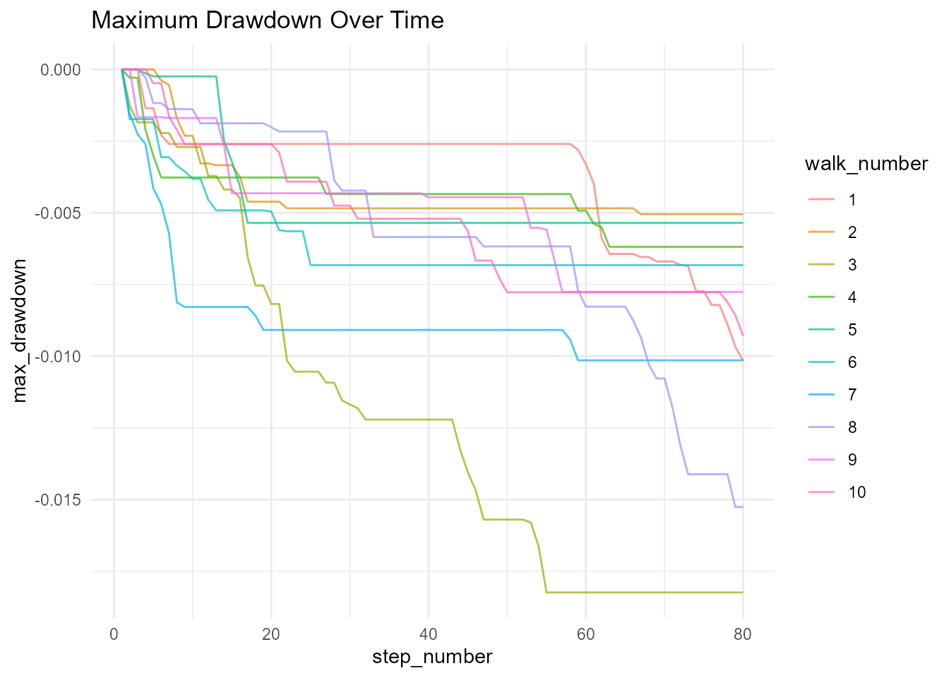

Line plot showing maximum drawdown over time for 10 random walks. Each walk is shown in a different color with semi-transparent lines. The y-axis shows the maximum drawdown as a negative percentage, and the x-axis shows the step number from 0 to 100.

Confidence Intervals

Using `confidence_interval()`

Calculate confidence intervals for a vector:

# Generate data
x <- rnorm(1000, mean = 10, sd = 2)

# Calculate 95% CI (default)
confidence_interval(x)
#> # A tibble: 1 × 2
#>   lower upper
#>   <dbl> <dbl>
#> 1  9.88  10.1

# Calculate 99% CI
confidence_interval(x, .interval = 0.01)
#> # A tibble: 1 × 2
#>   lower upper
#>   <dbl> <dbl>
#> 1 10.00  10.0

# Calculate 90% CI
confidence_interval(x, .interval = 0.10)
#> # A tibble: 1 × 2
#>   lower upper
#>   <dbl> <dbl>
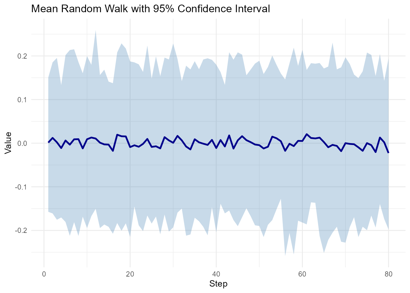
#> 1  9.99  10.0

Confidence Intervals for Random Walks

# Generate walks
walks <- random_normal_walk(.num_walks = 100, .n = 100)

# Calculate CI at each step
ci_by_step <- walks |>
  group_by(step_number) |>
  summarize(
    mean_val = mean(y),
    lower = quantile(y, 0.025),
    upper = quantile(y, 0.975)
  )

# Visualize
ggplot(ci_by_step, aes(x = step_number)) +
  geom_ribbon(aes(ymin = lower, ymax = upper), alpha = 0.3, fill = "steelblue") +
  geom_line(aes(y = mean_val), color = "darkblue", linewidth = 1) +
  theme_minimal() +
  labs(
    title = "Mean Random Walk with 95% Confidence Interval",
    x = "Step",
    y = "Value"
  )

Time series plot showing the mean random walk trajectory (dark blue line) surrounded by a light blue shaded region representing the 95% confidence interval. The x-axis shows step numbers from 0 to 100, and the y-axis shows the walk values.

Confidence Intervals for Final Values

# Get final values from many walks
walks <- random_normal_walk(.num_walks = 1000, .n = 100, .initial_value = 100)

final_values <- walks |>
  group_by(walk_number) |>
  slice_max(step_number, n = 1) |>
  pull(cum_sum_y)

# Calculate confidence interval
confidence_interval(final_values)
#> # A tibble: 1 × 2
#>   lower upper
#>   <dbl> <dbl>
#> 1 100.0  100.

Running Quantiles

Using `running_quantile()`

Calculate quantiles at each position:

# Generate walks
walks <- random_normal_walk(.num_walks = 100, .n = 100)

# Calculate running median (50th percentile)
walks_with_median <- walks |>
  group_by(step_number) |>
  mutate(median_at_step = running_quantile(y, .probs = 0.5, .window = 5)) |>
  ungroup()

# Show results
walks_with_median |>
  select(walk_number, step_number, y, median_at_step) |>
  head(10)
#> # A tibble: 10 × 4
#>    walk_number step_number        y median_at_step
#>    <fct>             <int>    <dbl>          <dbl>
#>  1 1                     1  0.123         0.000678
#>  2 1                     2  0.0201        0.0201  
#>  3 1                     3 -0.0235       -0.0235  
#>  4 1                     4 -0.0535       -0.0535  
#>  5 1                     5 -0.00384      -0.00384 
#>  6 1                     6 -0.122        -0.0440  
#>  7 1                     7 -0.0933       -0.0440  
#>  8 1                     8 -0.0562       -0.0562  
#>  9 1                     9  0.233        -0.0513  
#> 10 1                    10 -0.0647       -0.0647

# Calculate running quartiles
walks_with_quartiles <- walks |>
  group_by(step_number) |>
  mutate(
    q25 = running_quantile(y, .probs = 0.25, .window = 5),
    q50 = running_quantile(y, .probs = 0.50, .window = 5),
    q75 = running_quantile(y, .probs = 0.75, .window = 5)
  ) |>
  ungroup()

# Show results
walks_with_quartiles |>
  select(walk_number, step_number, y, q25, q50, q75) |>
  head(10)
#> # A tibble: 10 × 6
#>    walk_number step_number        y     q25       q50      q75
#>    <fct>             <int>    <dbl>   <dbl>     <dbl>    <dbl>
#>  1 1                     1  0.123   -0.0255  0.000678  0.0619 
#>  2 1                     2  0.0201   0.0151  0.0201    0.0238 
#>  3 1                     3 -0.0235  -0.0259 -0.0235    0.0187 
#>  4 1                     4 -0.0535  -0.0548 -0.0535    0.0653 
#>  5 1                     5 -0.00384 -0.0883 -0.00384   0.0308 
#>  6 1                     6 -0.122   -0.0831 -0.0440    0.00787
#>  7 1                     7 -0.0933  -0.0687 -0.0440   -0.0254 
#>  8 1                     8 -0.0562  -0.104  -0.0562    0.0533 
#>  9 1                     9  0.233   -0.0592 -0.0513    0.0906 
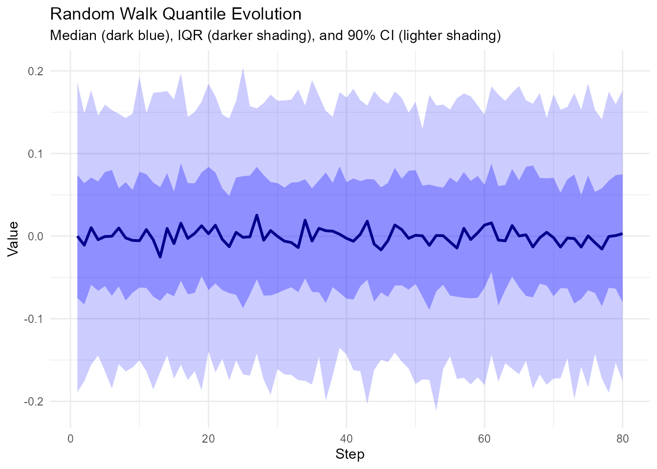
#> 10 1                    10 -0.0647  -0.125  -0.0647    0.0415

Visualizing Quantile Evolution

# Generate many walks
walks <- random_normal_walk(.num_walks = 200, .n = 100)

# Calculate quantiles at each step
quantile_evolution <- walks |>
  group_by(step_number) |>
  summarize(
    q05 = quantile(y, 0.05),
    q25 = quantile(y, 0.25),
    q50 = quantile(y, 0.50),
    q75 = quantile(y, 0.75),
    q95 = quantile(y, 0.95)
  )

# Plot
ggplot(quantile_evolution, aes(x = step_number)) +
  geom_ribbon(aes(ymin = q05, ymax = q95), alpha = 0.2, fill = "blue") +
  geom_ribbon(aes(ymin = q25, ymax = q75), alpha = 0.3, fill = "blue") +
  geom_line(aes(y = q50), color = "darkblue", linewidth = 1) +
  theme_minimal() +
  labs(
    title = "Random Walk Quantile Evolution",
    subtitle = "Median (dark blue), IQR (darker shading), and 90% CI (lighter shading)",
    x = "Step",
    y = "Value"
  )

Plot showing the evolution of quantiles over 100 steps for 200 random walks. A dark blue line shows the median (50th percentile), surrounded by darker blue shading showing the interquartile range (25th to 75th percentile), and lighter blue shading showing the 90% confidence interval (5th to 95th percentile). The x-axis shows step numbers and the y-axis shows walk values.

Distance Calculations

Using `euclidean_distance()`

For multi-dimensional walks, calculate distance from origin:

# 2D walk
walks_2d <- random_normal_walk(.num_walks = 10, .n = 100, .dimensions = 2)

# Calculate Euclidean distance
walks_with_distance <- walks_2d |>
  euclidean_distance(.x = x, .y = y)

# Visualize distance over time
walks_with_distance |>
  ggplot(aes(x = step_number, y = distance, color = walk_number)) +
  geom_line(alpha = 0.7) +
  theme_minimal() +
  labs(
    title = "Distance from Origin in 2D Random Walk",
    x = "Step",
    y = "Euclidean Distance"
  )
#> Warning: Removed 1 row containing missing values or values outside the scale range
#> (`geom_line()`).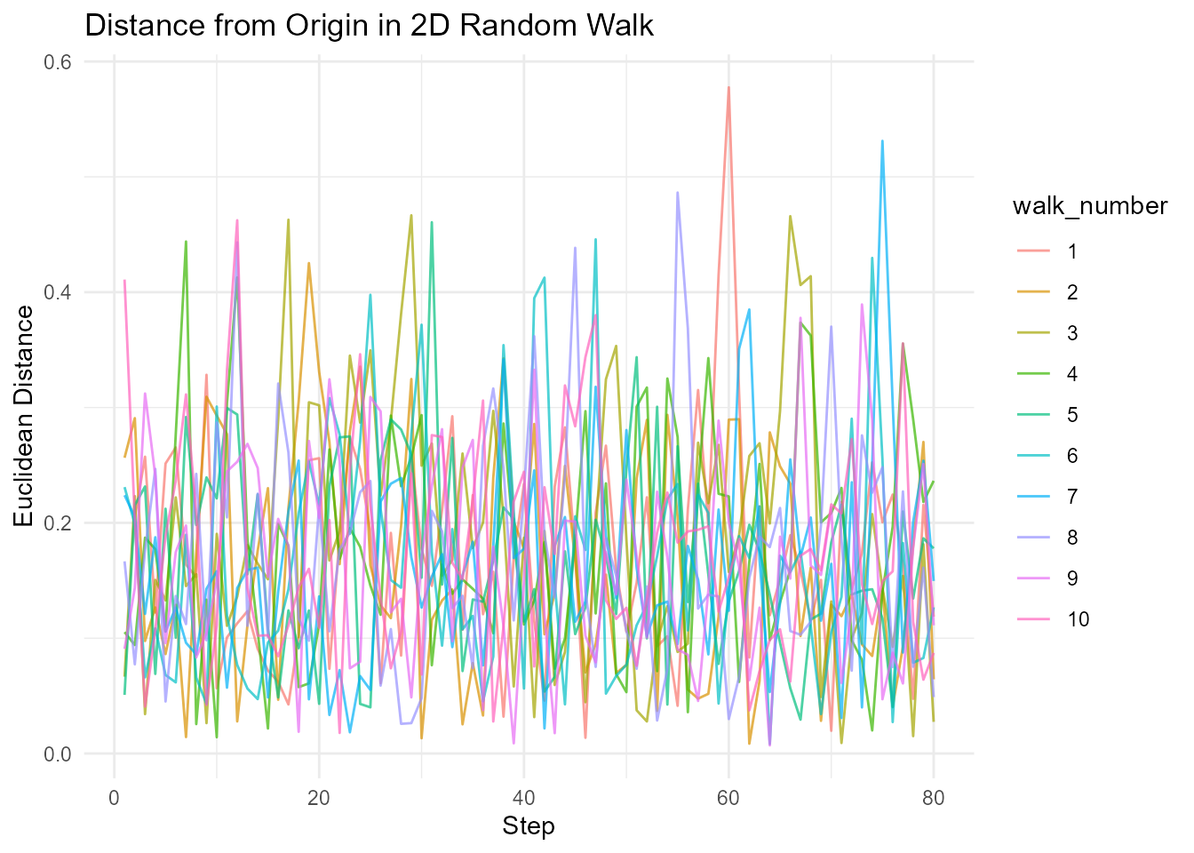

Multi-line plot showing Euclidean distance from origin over time for 10 different 2D random walks. Each walk is shown in a different color with semi-transparent lines. The x-axis shows step numbers from 0 to 100, and the y-axis shows the distance from the origin.

Distance Statistics

# 3D walk
walks_3d <- random_normal_walk(.num_walks = 100, .n = 1000, .dimensions = 3)

# Calculate distance
walks_with_dist <- walks_3d |> euclidean_distance(.x = x, .y = z)

# Analyze distance evolution
distance_stats <- walks_with_dist |>
  group_by(step_number) |>
  summarize(
    mean_dist = mean(distance),
    sd_dist = sd(distance),
    max_dist = max(distance)
  )

# Plot average distance vs sqrt(n) theoretical prediction
distance_stats |>
  ggplot(aes(x = step_number)) +
  geom_line(aes(y = mean_dist, color = "Observed"), linewidth = 1) +
  geom_line(aes(y = sqrt(3 * step_number), color = "Theory"), linewidth = 1, linetype = "dashed") +
  scale_color_manual(values = c("Observed" = "blue", "Theory" = "red")) +
  theme_minimal() +
  labs(
    title = "Mean Distance vs Theoretical Prediction",
    subtitle = "Distance ~ sqrt(3n) for 3D Brownian motion",
    x = "Step",
    y = "Distance",
    color = ""
  )
#> Warning: Removed 1 row containing missing values or values outside the scale range
#> (`geom_line()`).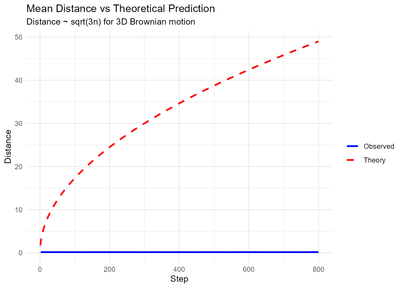

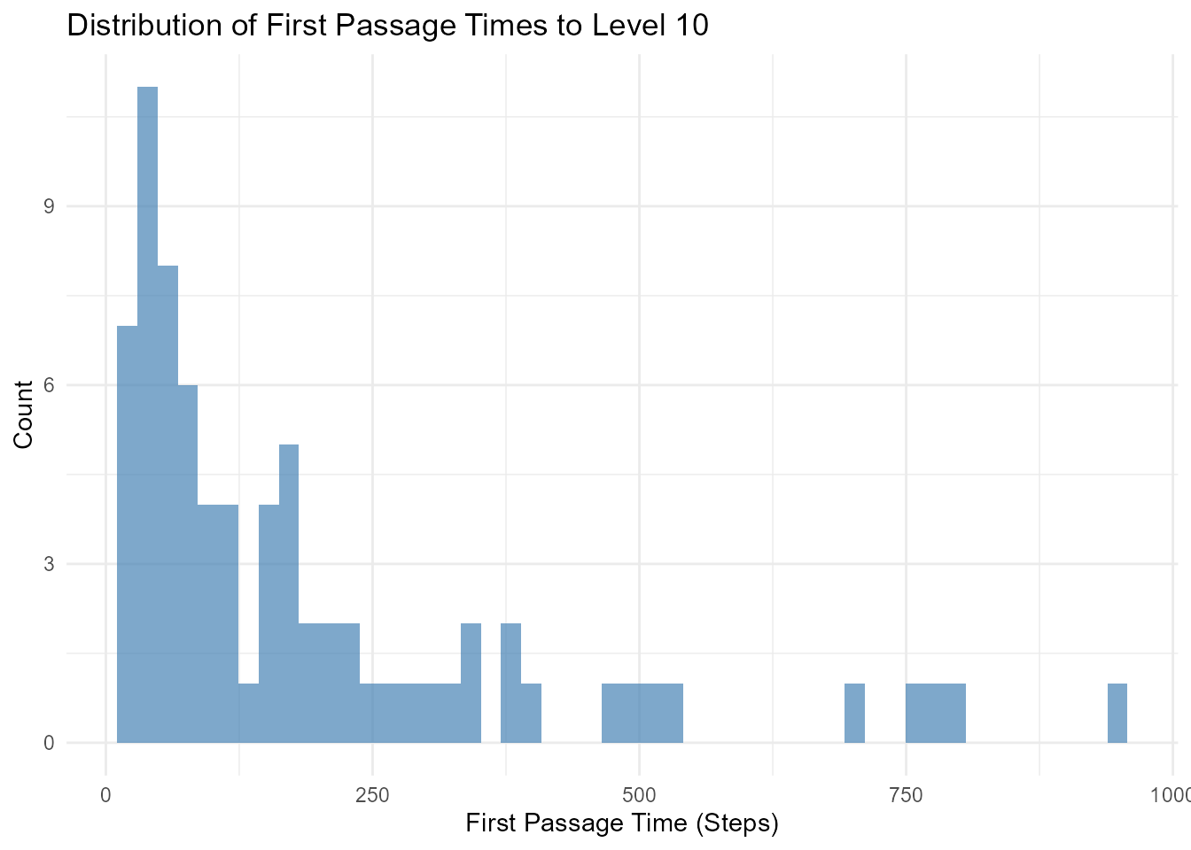
Line plot comparing observed mean distance (solid blue line) versus theoretical prediction (dashed red line) for 3D random walks. The theoretical prediction follows sqrt(n) as expected for standard Brownian motion. The x-axis shows step numbers and the y-axis shows distance from origin.

First Passage Time

Calculate when walks first reach a threshold:

# Generate walks
walks <- discrete_walk(.num_walks = 100, .n = 1000, .initial_value = 0)

# Find first passage time to level 10
first_passage <- walks |>
  group_by(walk_number) |>
  filter(cum_sum_y >= 10) |>
  slice_min(step_number, n = 1) |>
  select(walk_number, first_passage_time = step_number)

# Analyze distribution of first passage times
first_passage |>
  ggplot(aes(x = first_passage_time)) +
  geom_histogram(bins = 50, fill = "steelblue", alpha = 0.7) +
  theme_minimal() +
  labs(
    title = "Distribution of First Passage Times to Level 10",
    x = "First Passage Time (Steps)",
    y = "Count"
  )

Histogram showing the distribution of first passage times to level 10 for 100 discrete random walks. The x-axis shows the first passage time in steps, and the y-axis shows the count of walks. The distribution is right-skewed with most walks reaching level 10 within the first few hundred steps.

Subsetting Walks

Using `subset_walks()`

Extract walks with extreme values:

# Generate walks
walks <- random_normal_walk(.num_walks = 100, .n = 100, .initial_value = 100)

# Get walk with maximum final value
max_walk <- walks |> subset_walks(.value = "cum_sum_y", .type = "max")

# Get walk with minimum final value
min_walk <- walks |> subset_walks(.value = "cum_sum_y", .type = "min")

# Show the extreme walks
max_walk |> 
  summarize_walks(.value = cum_sum_y, .group_var = walk_number)
#> # A tibble: 1 × 17
#>   walk_number fns   fns_name   obs mean_val median range quantile_lo quantile_hi
#>   <fct>       <chr> <chr>    <int>    <dbl>  <dbl> <dbl>       <dbl>       <dbl>
#> 1 21          rand… Random …   100     101.   101.  2.86        100.        103.
#> # ℹ 8 more variables: variance <dbl>, sd <dbl>, min_val <dbl>, max_val <dbl>,
#> #   harmonic_mean <dbl>, geometric_mean <dbl>, skewness <dbl>, kurtosis <dbl>

min_walk |> 
  summarize_walks(.value = cum_sum_y, .group_var = walk_number)
#> # A tibble: 1 × 17
#>   walk_number fns   fns_name   obs mean_val median range quantile_lo quantile_hi
#>   <fct>       <chr> <chr>    <int>    <dbl>  <dbl> <dbl>       <dbl>       <dbl>
#> 1 66          rand… Random …   100     98.3   98.3  2.84        97.2        99.8
#> # ℹ 8 more variables: variance <dbl>, sd <dbl>, min_val <dbl>, max_val <dbl>,
#> #   harmonic_mean <dbl>, geometric_mean <dbl>, skewness <dbl>, kurtosis <dbl>

Finding Specific Walks

# Find walks that cross a threshold
walks <- random_normal_walk(.num_walks = 100, .n = 100, .initial_value = 100)

# Identify walks that reached 102
crossed_102 <- walks |>
  group_by(walk_number) |>
  filter(any(cum_sum_y >= 102)) |>
  pull(walk_number) |>
  unique()

# Extract and visualize those walks
walks |>
  filter(walk_number %in% crossed_102) |>
  visualize_walks(.pluck = "cum_sum", .alpha = 0.3)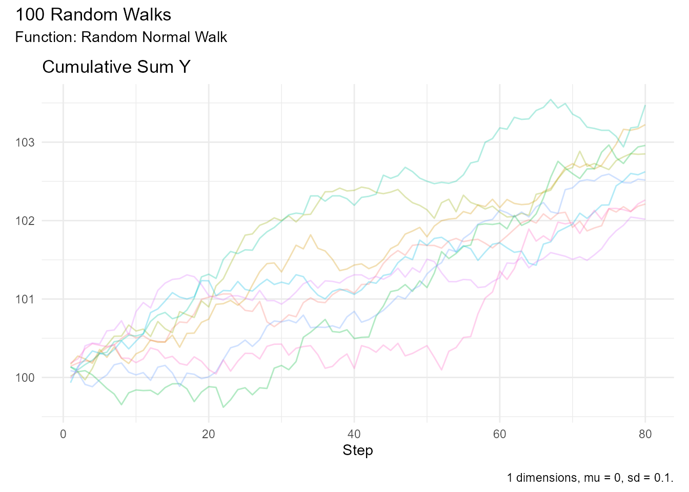

Multi-line plot showing all random walks that crossed the threshold of 102 at some point during their evolution. Multiple semi-transparent lines in different colors show the cumulative sum trajectories. The x-axis shows step numbers from 0 to 100, and the y-axis shows the cumulative sum values.

Advanced Analysis

Autocorrelation Analysis

# Generate walk with drift
walks <- random_normal_drift_walk(.num_walks = 1, .n = 500, .mu = 0.1)

# Calculate autocorrelation
acf_result <- walks |> pull(y) |> acf(plot = FALSE)

# Plot
plot(acf_result, main = "Autocorrelation of Random Walk Steps")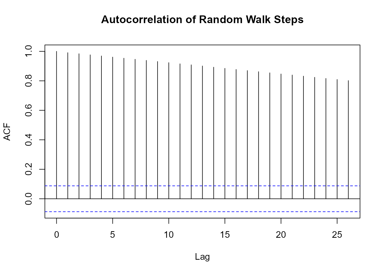

Autocorrelation function (ACF) plot showing the correlation of random walk steps with their lagged values. Vertical bars represent correlation values at different lags, with dashed blue lines indicating significance thresholds.

Distribution Testing

# Generate walks
walks <- random_normal_walk(.num_walks = 100, .n = 100)

# Test if steps are normally distributed
steps <- walks |> pull(y)

# Shapiro-Wilk test for normality
shapiro.test(sample(steps, 5000))  # Sample for computational efficiency
#> 
#>  Shapiro-Wilk normality test
#> 
#> data:  sample(steps, 5000)
#> W = 0.99943, p-value = 0.1313

# Q-Q plot
qqnorm(steps)
qqline(steps)

Q-Q (quantile-quantile) plot comparing the distribution of random walk steps to a theoretical normal distribution. Points falling along the diagonal reference line indicate good agreement with normality.

Variance Ratio Test

Test for random walk hypothesis:

# Generate walk
walk <- random_normal_walk(.num_walks = 1, .n = 1000)

# Calculate variance ratio
values <- walk |> pull(cum_sum_y)

# Variance of k-differences
k <- 10
var_k <- var(diff(values, lag = k))
var_1 <- var(diff(values, lag = 1))

# Variance ratio (should be ≈ k for random walk)
vr <- var_k / (k * var_1)
print(paste("Variance Ratio:", round(vr, 3), "| Expected:", k))
#> [1] "Variance Ratio: 1.014 | Expected: 10"

Return Analysis (Financial)

# Generate stock price simulation
prices <- geometric_brownian_motion(
  .num_walks = 1,
  .n = 252,
  .mu = 0.08,
  .sigma = 0.25,
  .initial_value = 100
)

# Calculate returns
returns <- prices |>
  mutate(
    log_return = log(cum_prod_y / lag(cum_prod_y)),
    simple_return = (cum_prod_y - lag(cum_prod_y)) / lag(cum_prod_y)
  ) |>
  filter(!is.na(log_return))

# Analyze returns
returns |>
  summarize(
    mean_return = mean(log_return) * 252,  # Annualized
    volatility = sd(log_return) * sqrt(252),  # Annualized
    sharpe_ratio = mean_return / volatility
  )
#> # A tibble: 1 × 3
#>   mean_return volatility sharpe_ratio
#>         <dbl>      <dbl>        <dbl>
#> 1        144.      0.928         155.

Statistical Tests

Comparing Distributions

# Generate two types of walks
normal_walks <- random_normal_walk(.num_walks = 50, .n = 100)
cauchy_walks <- random_cauchy_walk(.num_walks = 50, .n = 100)

# Get final values
normal_final <- normal_walks |>
  group_by(walk_number) |>
  slice_max(step_number) |>
  pull(cum_sum_y)

cauchy_final <- cauchy_walks |>
  group_by(walk_number) |>
  slice_max(step_number) |>
  pull(cum_sum_y)

# Wilcoxon rank-sum test (non-parametric)
wilcox.test(normal_final, cauchy_final)
#> 
#>  Wilcoxon rank sum test with continuity correction
#> 
#> data:  normal_final and cauchy_final
#> W = 1266, p-value = 0.9149
#> alternative hypothesis: true location shift is not equal to 0

# Kolmogorov-Smirnov test
ks.test(normal_final, cauchy_final)
#> 
#>  Exact two-sample Kolmogorov-Smirnov test
#> 
#> data:  normal_final and cauchy_final
#> D = 0.48, p-value = 1.387e-05
#> alternative hypothesis: two-sided

Testing for Drift

# Generate walk with known drift
walks <- random_normal_drift_walk(.num_walks = 100, .n = 100, .mu = 0.1)

# Test if mean step is significantly different from 0
steps <- walks |> pull(y)
t.test(steps, mu = 0)
#> 
#>  One Sample t-test
#> 
#> data:  steps
#> t = 115.67, df = 9999, p-value < 2.2e-16
#> alternative hypothesis: true mean is not equal to 0
#> 95 percent confidence interval:
#>  10.10977 10.45834
#> sample estimates:
#> mean of x 
#>  10.28405

Next Steps

Visualization Guide - Visualize your analysis
Use Cases and Examples - Real-world applications
Multi-Dimensional Walks - Analyze spatial walks
API Reference - Complete function documentation

Need more examples? Check out the Use Cases and Examples vignette for more real-world applications!

Table of Contents