Bootstrap Analysis

set.seed(123)
library(TidyDensity)
library(dplyr)
library(ggplot2)
library(patchwork)

Bootstrap resampling is a powerful statistical technique for robust inference. TidyDensity provides integrated bootstrap functionality with seamless visualization and analysis tools.

What is Bootstrap?

Concept

Bootstrap resampling is a non-parametric method for:

• Estimating sampling distributions
• Calculating confidence intervals
• Assessing parameter uncertainty
• Making inferences without distributional assumptions

How It Works

1. Resample your data with replacement
2. Calculate statistic of interest for each resample
3. Repeat process many times (typically 1000-10000)
4. Analyze distribution of bootstrap statistics

When to Use Bootstrap

• Unknown or complex sampling distributions
• Small to medium sample sizes
• When parametric assumptions are questionable
• For robust confidence intervals
• Complex statistics (median, trimmed mean, etc.)

Bootstrap in TidyDensity

Main Function: tidy_bootstrap()

Generate bootstrap samples in tidy format:

tidy_bootstrap(
  .x,                    # Your data vector
  .num_sims = 2000,      # Number of bootstrap samples
  .proportion = 0.8,     # Proportion to sample (default = 0.8)
  .distribution_type = "continuous"  # continuous or discrete
)

Return Value

Returns a tidy tibble with:

• sim_number - Bootstrap sample identifier
• bootstrap_samples - List column of bootstrap samples of .x

Basic Bootstrap Analysis

Simple Bootstrap Example

# Your data
data <- mtcars$mpg

# Perform bootstrap
bootstrap_data <- tidy_bootstrap(
  .x = data,
  .num_sims = 2000
)

# View structure
head(bootstrap_data)
#> # A tibble: 6 × 2
#>   sim_number bootstrap_samples
#>   <fct>      <list>           
#> 1 1          <dbl [25]>       
#> 2 2          <dbl [25]>       
#> 3 3          <dbl [25]>       
#> 4 4          <dbl [25]>       
#> 5 5          <dbl [25]>       
#> 6 6          <dbl [25]>

Visualizing Bootstrap Distribution

# Density plot of bootstrap distribution Cumulative Mean
bootstrap_stat_plot(bootstrap_data, .value = y, .stat = "cmean")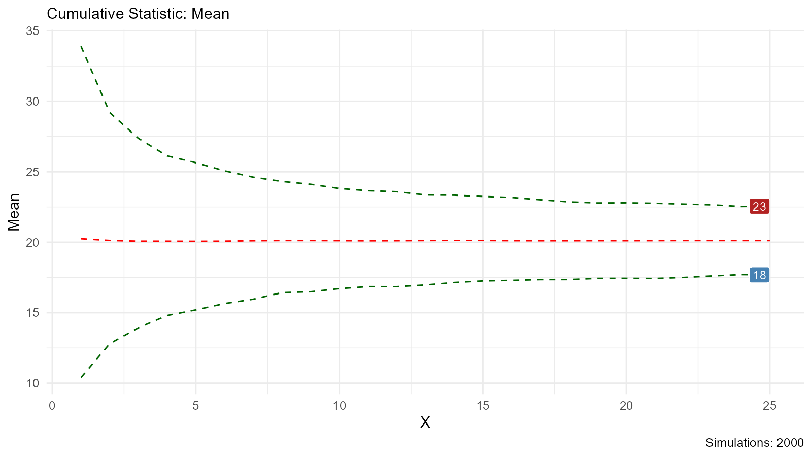

# Cumulative Harmonic Mean
bootstrap_stat_plot(bootstrap_data, .value = y, .stat = "chmean")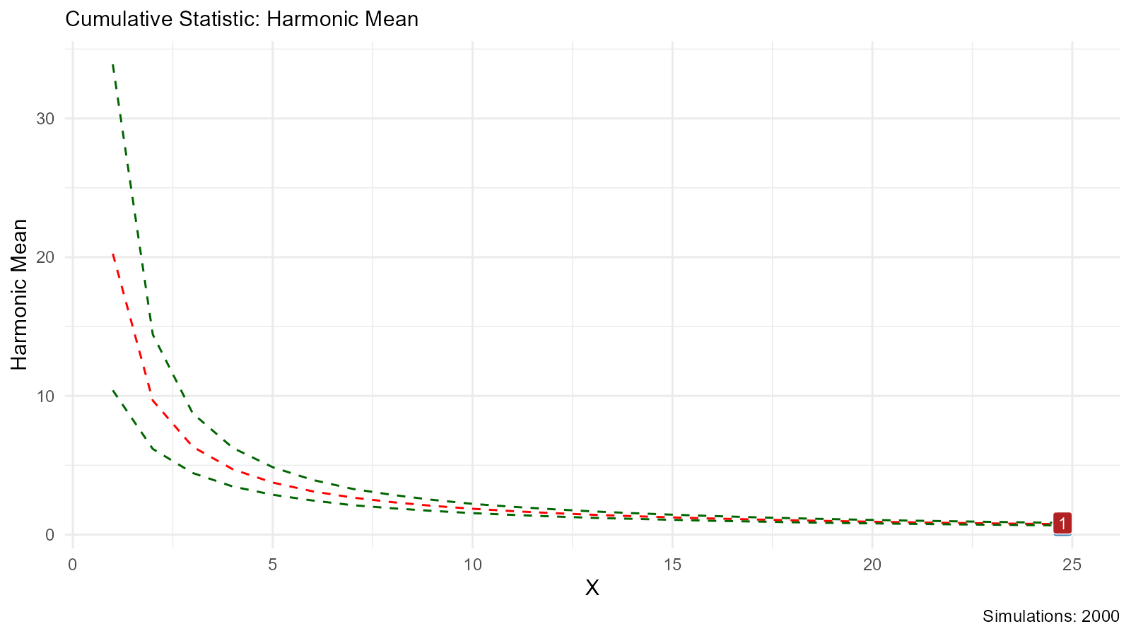

# Show Groups
bootstrap_stat_plot(bootstrap_data, .value = y, .stat = "cmean",
                    .show_groups = TRUE)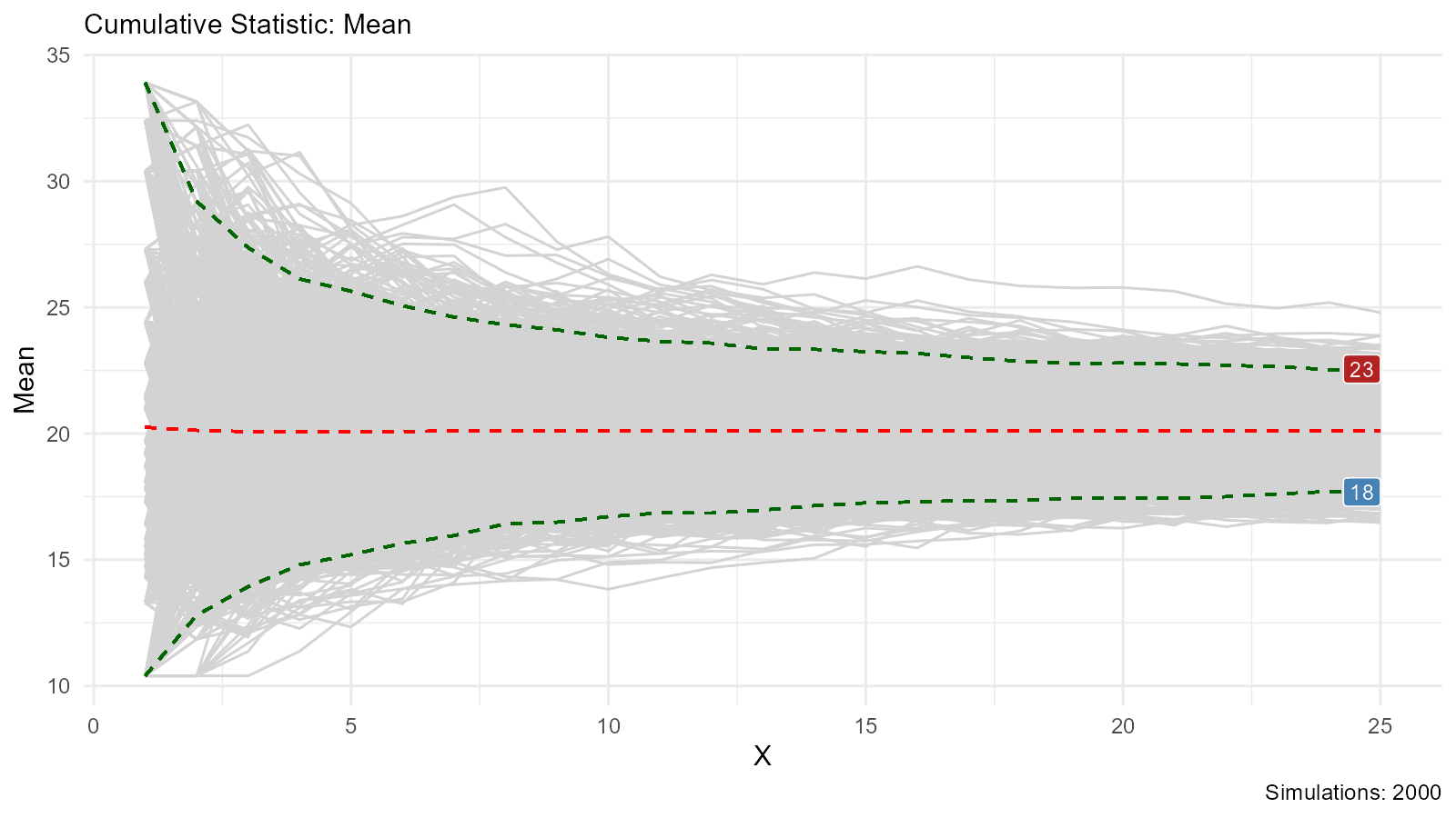

Quick Statistics

# Get basic statistics
summary(bootstrap_data |> bootstrap_unnest_tbl() |> pull(y))
#>    Min. 1st Qu.  Median    Mean 3rd Qu.    Max. 
#>   10.40   15.50   19.20   20.12   22.80   33.90

# Count simulations
length(unique(bootstrap_data$sim_number))
#> [1] 2000

Bootstrap Statistics

Unnesting Bootstrap Data

Use bootstrap_unnest_tbl() to work with bootstrap samples:

# Unnest the bootstrap data
unnested <- bootstrap_data |>
  bootstrap_unnest_tbl()

# Now you can calculate statistics
head(unnested)
#> # A tibble: 6 × 2
#>   sim_number     y
#>   <fct>      <dbl>
#> 1 1           15  
#> 2 1           10.4
#> 3 1           30.4
#> 4 1           15.2
#> 5 1           22.8
#> 6 1           19.2

Calculating Bootstrap Statistics

# Calculate statistics for each bootstrap sample
bootstrap_stats <- bootstrap_data |>
  bootstrap_unnest_tbl() |>
  group_by(sim_number) |>
  summarise(
    mean = mean(y),
    median = median(y),
    sd = sd(y),
    q25 = quantile(y, 0.25),
    q75 = quantile(y, 0.75)
  )

# View distribution of means
summary(bootstrap_stats$mean)
#>    Min. 1st Qu.  Median    Mean 3rd Qu.    Max. 
#>   16.47   19.34   20.09   20.12   20.91   24.79
hist(bootstrap_stats$mean, main = "Bootstrap Distribution of Mean",
     xlab = "Mean", col = "lightblue")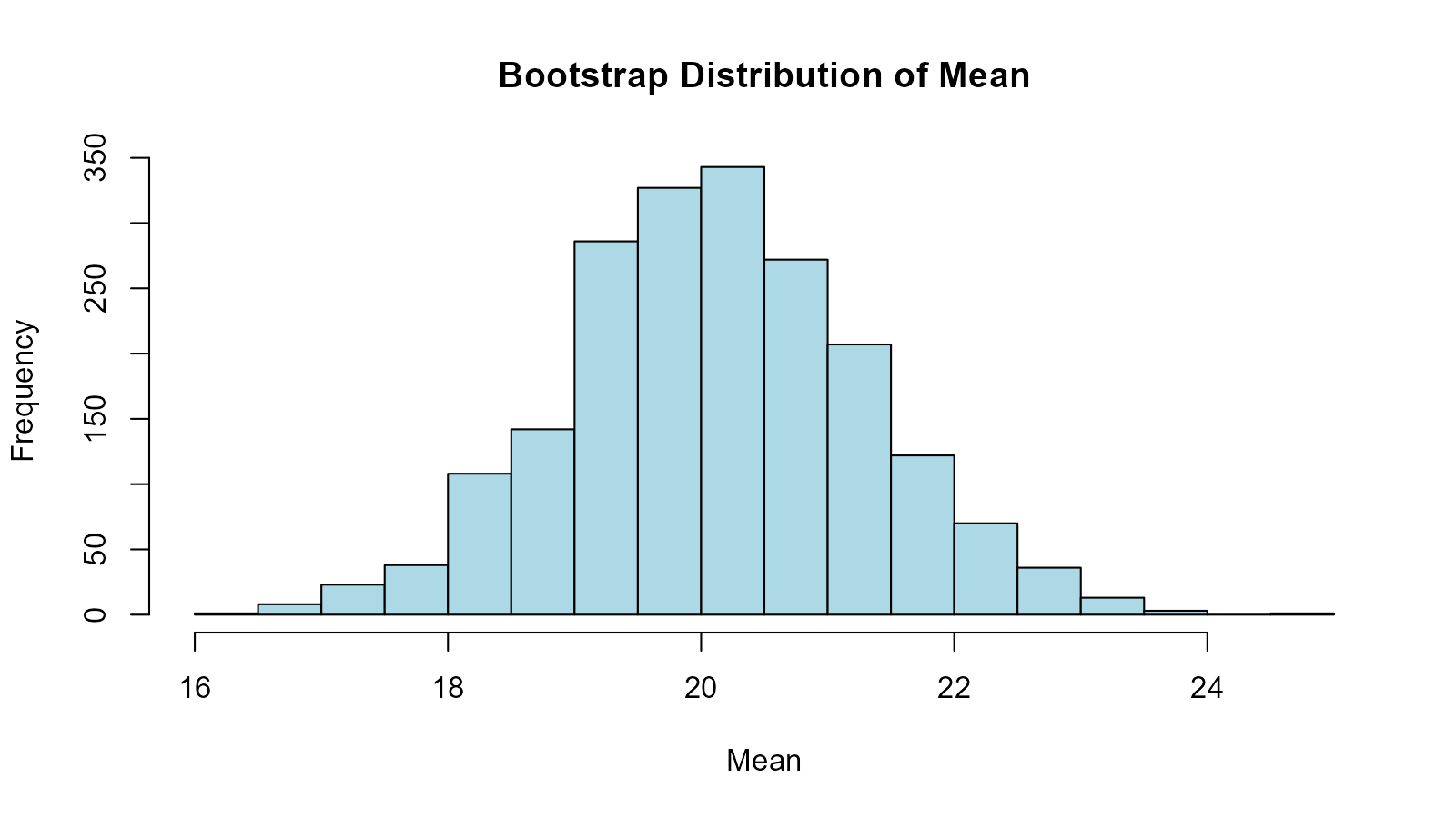

Overall Bootstrap Statistics

# Calculate overall statistics from all bootstrap samples
overall_stats <- bootstrap_data |>
  bootstrap_unnest_tbl() |>
  summarise(
    mean_est = mean(y),
    sd_est = sd(y),
    median_est = median(y)
  )

overall_stats
#> # A tibble: 1 × 3
#>   mean_est sd_est median_est
#>      <dbl>  <dbl>      <dbl>
#> 1     20.1   5.94       19.2

Confidence Intervals

Bootstrap Percentile Method

Most common and intuitive method:

# Calculate 95% confidence intervals
ci_level <- 0.95
alpha <- 1 - ci_level

bootstrap_ci <- bootstrap_data |>
  bootstrap_unnest_tbl() |>
  summarise(
    lower_ci = quantile(y, alpha/2),
    upper_ci = quantile(y, 1 - alpha/2),
    point_estimate = mean(y)
  )

bootstrap_ci
#> # A tibble: 1 × 3
#>   lower_ci upper_ci point_estimate
#>      <dbl>    <dbl>          <dbl>
#> 1     10.4     33.9           20.1

Confidence Intervals for Multiple Statistics

# Calculate CI for mean, median, and sd
ci_stats <- bootstrap_data |>
  bootstrap_unnest_tbl() |>
  group_by(sim_number) |>
  summarise(
    mean = mean(y),
    median = median(y),
    sd = sd(y)
  ) |>
  summarise(
    across(
      c(mean, median, sd),
      list(
        lower = ~ unname(quantile(.x, 0.025)),
        estimate = ~ unname(mean(.x)),
        upper = ~ unname(quantile(.x, 0.975))
      )
    )
  )

glimpse(ci_stats)
#> Rows: 1
#> Columns: 9
#> $ mean_lower      <dbl> 17.6837
#> $ mean_estimate   <dbl> 20.11925
#> $ mean_upper      <dbl> 22.5564
#> $ median_lower    <dbl> 16.4
#> $ median_estimate <dbl> 19.28125
#> $ median_upper    <dbl> 21.4025
#> $ sd_lower        <dbl> 4.104046
#> $ sd_estimate     <dbl> 5.879158
#> $ sd_upper        <dbl> 7.384673

Visualizing Confidence Intervals

# Create visualization
unnested |>
  ggplot(aes(x = y)) +
  geom_density(fill = "lightblue", alpha = 0.5) +
  geom_vline(xintercept = unname(quantile(unnested$y, 0.025)), 
             linetype = "dashed", color = "red") +
  geom_vline(xintercept = unname(quantile(unnested$y, 0.975)), 
             linetype = "dashed", color = "red") +
  geom_vline(xintercept = mean(unnested$y), 
             linetype = "solid", color = "darkblue", linewidth = 1) +
  labs(
    title = "Bootstrap Distribution with 95% CI",
    x = "Bootstrap Statistic",
    y = "Density"
  ) +
  theme_minimal()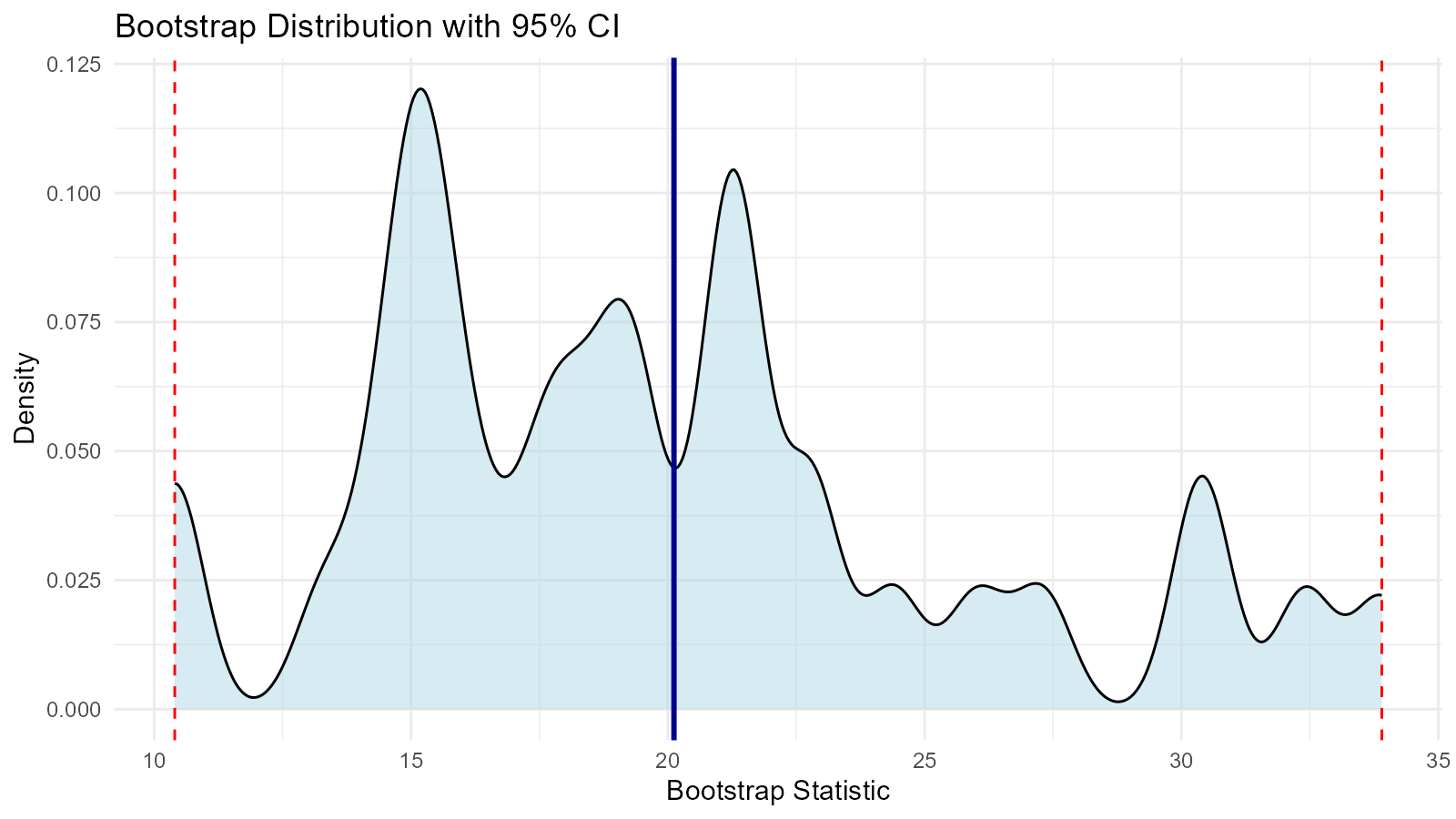

Bootstrap Augmentation Functions

Augment Density

Add density calculations to bootstrap data:

# Augment with density information
augmented_density <- bootstrap_data |>
  bootstrap_density_augment()

head(augmented_density)
#> # A tibble: 6 × 5
#>   sim_number     x     y    dx        dy
#>   <fct>      <int> <dbl> <dbl>     <dbl>
#> 1 1              1  15    1.30 0.0000593
#> 2 1              2  10.4  3.04 0.000286 
#> 3 1              3  30.4  4.78 0.00102  
#> 4 1              4  15.2  6.51 0.00279  
#> 5 1              5  22.8  8.25 0.00624  
#> 6 1              6  19.2  9.99 0.0124

Augment Probability

Add cumulative probability:

# Augment with probability information
augmented_prob <- bootstrap_data |>
  bootstrap_unnest_tbl() |>
  bootstrap_p_augment(y)

head(augmented_prob)
#> # A tibble: 6 × 3
#>   sim_number     y      p
#>   <fct>      <dbl>  <dbl>
#> 1 1           15   0.186 
#> 2 1           10.4 0.0618
#> 3 1           30.4 0.937 
#> 4 1           15.2 0.249 
#> 5 1           22.8 0.779 
#> 6 1           19.2 0.530

Augment Quantile

Add quantile information:

# Augment with quantile information
augmented_quantile <- bootstrap_data |>
  bootstrap_unnest_tbl() |>
  bootstrap_q_augment(y)

head(augmented_quantile)
#> # A tibble: 6 × 3
#>   sim_number     y     q
#>   <fct>      <dbl> <dbl>
#> 1 1           15    10.4
#> 2 1           10.4  10.4
#> 3 1           30.4  10.4
#> 4 1           15.2  10.4
#> 5 1           22.8  10.4
#> 6 1           19.2  10.4

Advanced Bootstrap Techniques

Bootstrap for Difference of Means

# Two groups
group1 <- mtcars$mpg[mtcars$am == 0]
group2 <- mtcars$mpg[mtcars$am == 1]

# Bootstrap function for difference
bootstrap_diff <- function(n_sims = 2000) {
  diffs <- numeric(n_sims)
  
  for (i in 1:n_sims) {
    boot_g1 <- sample(group1, length(group1), replace = TRUE)
    boot_g2 <- sample(group2, length(group2), replace = TRUE)
    diffs[i] <- mean(boot_g2) - mean(boot_g1)
  }
  
  return(diffs)
}

# Run bootstrap
diff_dist <- bootstrap_diff(2000)

# Calculate CI
quantile(diff_dist, c(0.025, 0.975))
#>      2.5%     97.5% 
#>  3.827439 10.924939

# Visualize
hist(diff_dist, main = "Bootstrap Distribution of Difference in Means",
     xlab = "Difference in Means", breaks = 50, col = "lightgreen")
abline(v = quantile(diff_dist, c(0.025, 0.975)), 
       col = "red", lty = 2, lwd = 2)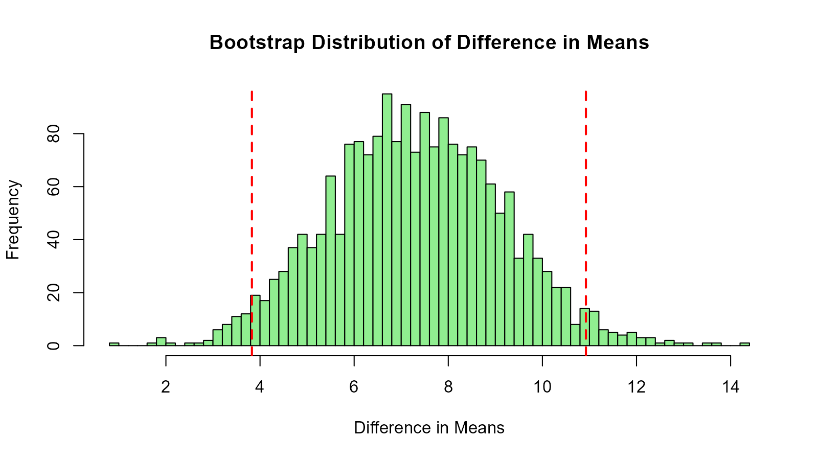

Bootstrap for Correlation

# Original correlation
cor_original <- cor(mtcars$mpg, mtcars$wt)

# Bootstrap correlations
boot_cor <- function(x, y, n_sims = 2000) {
  cors <- numeric(n_sims)
  n <- length(x)
  
  for (i in 1:n_sims) {
    indices <- sample(n, replace = TRUE)
    cors[i] <- cor(x[indices], y[indices])
  }
  
  return(cors)
}

# Run bootstrap
cor_dist <- boot_cor(mtcars$mpg, mtcars$wt, 2000)

# CI for correlation
cor_ci <- quantile(cor_dist, c(0.025, 0.975))
cat("95% CI for correlation:", cor_ci, "\n")
#> 95% CI for correlation: -0.9276411 -0.7921946

# Visualize
hist(cor_dist, main = "Bootstrap Distribution of Correlation",
     xlab = "Correlation Coefficient", breaks = 50, col = "lightyellow")
abline(v = cor_ci, col = "red", lty = 2, lwd = 2)
abline(v = cor_original, col = "blue", lwd = 2)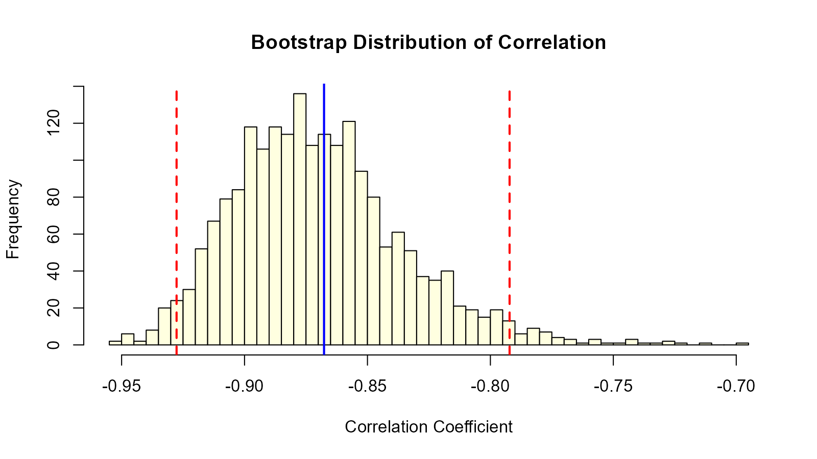

Visualization

Multiple Visualizations

# Generate bootstrap data
boot_data <- tidy_bootstrap(mtcars$mpg, .num_sims = 2000) |>
  bootstrap_unnest_tbl()

# Create multiple plots
p1 <- ggplot(aes(x = y), data = boot_data) +
  geom_density(fill = "lightgreen", alpha = 0.5) +
  labs(title = "Density Plot", x = "Value", y = "Density") +
  theme_minimal()

p2 <- ggplot(aes(x = y), data = boot_data) +
  stat_ecdf(aes(x = y), geom = "step", color = "blue") +
  labs(title = "Probability Plot", x = "Value", y = "Cumulative Probability") +
  theme_minimal()

p3 <- ggplot(aes(x = seq_along(y), y = sort(y)), data = boot_data) +
  geom_point(color = "purple", alpha = 0.1) +
  labs(title = "Sorted Values", x = "Index", y = "Value") +
  theme_minimal()

p4 <- ggplot(aes(sample = y), data = boot_data) +
  stat_qq(color = "orange", alpha = 0.1) +
  stat_qq_line(color = "red") +
  labs(title = "QQ Plot", x = "Theoretical Quantiles", y = "Sample Quantiles") +
  theme_minimal()

# Combine
(p1 | p2) / (p3 | p4)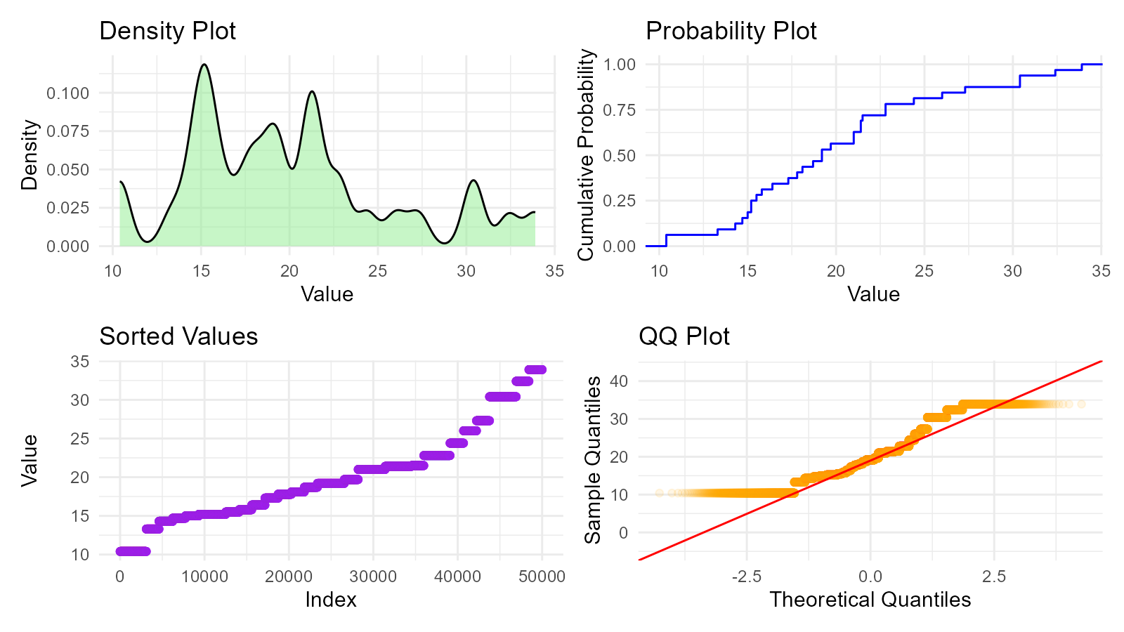

Custom Visualization with CI

# Calculate statistics
ci <- quantile(boot_data$y, c(0.025, 0.5, 0.975))

# Create plot
ggplot(data.frame(y = boot_data$y), aes(x = y)) +
  geom_density(fill = "skyblue", alpha = 0.5) +
  geom_vline(xintercept = ci[1], linetype = "dashed", color = "red") +
  geom_vline(xintercept = ci[2], linetype = "solid", color = "darkblue", 
             linewidth = 1.5) +
  geom_vline(xintercept = ci[3], linetype = "dashed", color = "red") +
  annotate("text", x = ci[1], y = 0, label = "2.5%", vjust = -1) +
  annotate("text", x = ci[2], y = 0, label = "Median", vjust = -1) +
  annotate("text", x = ci[3], y = 0, label = "97.5%", vjust = -1) +
  labs(
    title = "Bootstrap Distribution with Confidence Interval",
    x = "Statistic Value",
    y = "Density"
  ) +
  theme_minimal()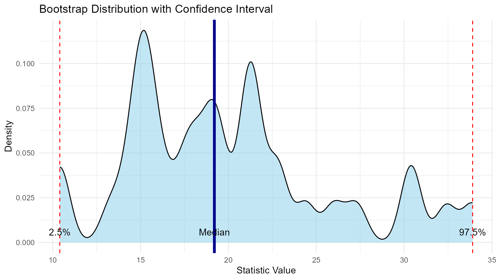

Best Practices

1. Choose Appropriate Number of Simulations

General guidelines:

• Exploratory: 1000 simulations
• Standard analysis: 2000-5000 simulations
• Publication/Critical: 10000+ simulations

2. Verify Bootstrap Convergence

Check stability with different numbers of simulations:

# Check stability with different numbers of simulations
n_sims_vec <- c(500, 1000, 2000)
convergence <- data.frame(
  n_sims = n_sims_vec,
  mean_est = NA,
  ci_lower = NA,
  ci_upper = NA
)

for (i in seq_along(n_sims_vec)) {
  boot <- tidy_bootstrap(data, .num_sims = n_sims_vec[i])
  stats <- boot |>
    bootstrap_unnest_tbl() |>
    summarise(
      mean = mean(y),
      lower = quantile(y, 0.025),
      upper = quantile(y, 0.975)
    )
  
  convergence[i, 2:4] <- as.numeric(stats)
}

convergence
#>   n_sims mean_est ci_lower ci_upper
#> 1    500 20.11131     10.4     33.9
#> 2   1000 20.06232     10.4     33.9
#> 3   2000 20.07139     10.4     33.9

3. Consider Sample Size

Bootstrap reliability depends on sample size:

n <- length(data)

if (n < 20) {
  message("Small sample size. Bootstrap may be less reliable.")
  message("Consider: n >= 30 for bootstrap")
}

cat("Sample size:", n, "\n")
#> Sample size: 32

4. Understand Limitations

Bootstrap works well for:

• Means, medians, quantiles
• Standard errors
• Confidence intervals

Bootstrap may struggle with:

• Extreme values (min/max)
• Very small samples
• Heavily dependent data
• Some complex statistics

Troubleshooting

Issue: CI Too Wide

Causes:

• High variability in data
• Small sample size
• Insufficient bootstrap samples

Solutions:

• Increase bootstrap samples
• Check data variability with coefficient of variation: sd(data) / mean(data)
• Collect more data if possible

Issue: Long Computation Time

Solutions:

• Reduce number of simulations for exploration
• Use parallel processing for large-scale analysis