Parameter Estimation

set.seed(123)
library(TidyDensity)
library(dplyr)
library(ggplot2)

TidyDensity provides comprehensive parameter estimation capabilities to fit probability distributions to empirical data using multiple statistical methods.

Overview

Parameter estimation allows you to:

• Fit distributions to your empirical data
• Estimate distribution parameters from observed values
• Compare theoretical vs empirical distributions
• Select best-fitting distribution using AIC
• Validate distributional assumptions

General Pattern

All parameter estimation functions follow this pattern:

util_[distribution]_param_estimate(
  .x,                           # Your data vector
  .auto_gen_empirical = TRUE    # Auto-generate comparison data
)

Estimation Methods

TidyDensity uses three primary estimation methods:

1. Maximum Likelihood Estimation (MLE)

What it is:

• Finds parameters that maximize the likelihood of observing your data
• Most commonly used method
• Asymptotically efficient

When to use:

• Large sample sizes (n > 30)
• When you need optimal statistical properties
• Default choice for most applications

Characteristics:

• Asymptotically unbiased
• Minimum variance for large samples
• Requires iterative computation

2. Method of Moments Estimation (MME)

What it is:

• Matches sample moments (mean, variance) to theoretical moments
• Often produces same results as MLE for common distributions
• Computationally simpler

When to use:

• Quick approximations needed
• Educational purposes
• When MLE is computationally expensive

Characteristics:

• Easy to compute
• Intuitive interpretation
• May be less efficient than MLE

3. Minimum Variance Unbiased Estimation (MVUE)

What it is:

• Provides unbiased estimates with minimum variance
• Uses correction factors for small samples
• Often same as MLE for large samples

When to use:

• Small sample sizes
• When unbiasedness is critical
• Comparing with MLE

Characteristics:

• Unbiased for any sample size
• Minimum variance among unbiased estimators
• May differ from MLE for small samples

Basic Usage

Simple Parameter Estimation

# Your empirical data
data <- mtcars$mpg

# Estimate normal distribution parameters
result <- util_normal_param_estimate(data, .auto_gen_empirical = TRUE)

# View parameter estimates
result$parameter_tbl
#> # A tibble: 2 × 8
#>   dist_type samp_size   min   max method              mu stan_dev shape_ratio
#>   <chr>         <int> <dbl> <dbl> <chr>            <dbl>    <dbl>       <dbl>
#> 1 Gaussian         32  10.4  33.9 EnvStats_MME_MLE  20.1     5.93        3.39
#> 2 Gaussian         32  10.4  33.9 EnvStats_MVUE     20.1     6.03        3.33

Understanding the Output

The function returns a list with several components including parameter estimates from different methods.

Visualizing the Fit

# Plot empirical vs fitted distribution
result$combined_data_tbl |>
  tidy_combined_autoplot()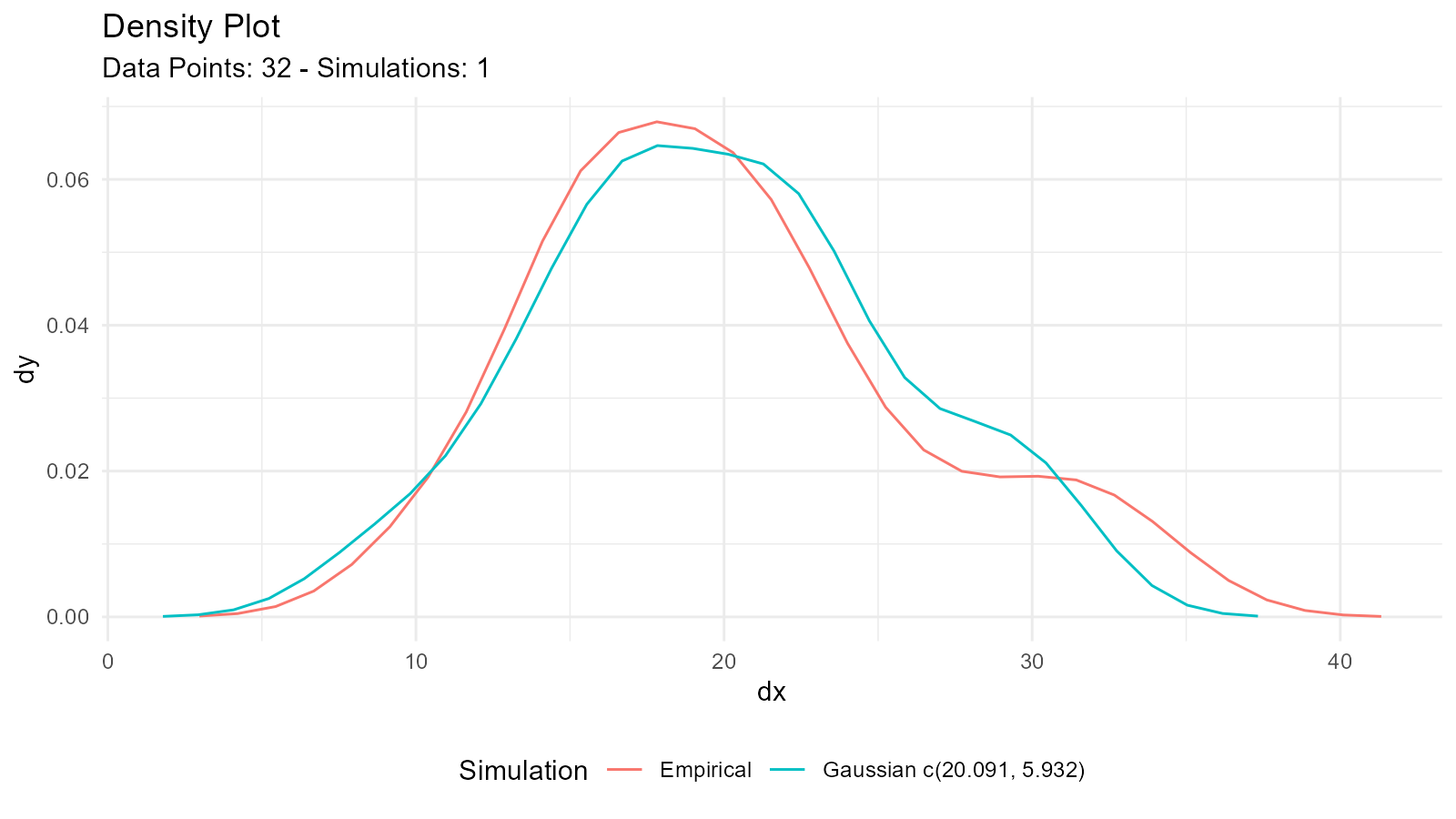

This creates a plot comparing:

• Your empirical data (density plot)
• Fitted distribution from MLE/MME
• Fitted distribution from MVUE

Comparing Methods

Example: Normal Distribution

# Generate some sample data
sample_data <- rnorm(100, mean = 50, sd = 10)

# Estimate parameters
estimates <- util_normal_param_estimate(sample_data)

# View both methods
estimates$parameter_tbl
#> # A tibble: 2 × 8
#>   dist_type samp_size   min   max method              mu stan_dev shape_ratio
#>   <chr>         <int> <dbl> <dbl> <chr>            <dbl>    <dbl>       <dbl>
#> 1 Gaussian        100  26.9  71.9 EnvStats_MME_MLE  50.4     8.67        5.81
#> 2 Gaussian        100  26.9  71.9 EnvStats_MVUE     50.4     8.71        5.78

Understanding Differences

For Normal Distribution:

• MLE/MME: Uses sample standard deviation with n-1 denominator
• MVUE: Corrects for bias in small samples

When n is large: MLE and MVUE converge

When n is small: MVUE provides better unbiased estimate

Example: Gamma Distribution

# Generate gamma-distributed data
sample_data <- rgamma(50, shape = 2, rate = 0.5)

# Estimate parameters
estimates <- util_gamma_param_estimate(sample_data, .auto_gen_empirical = TRUE)

# Compare estimates
estimates$parameter_tbl
#> # A tibble: 3 × 10
#>   dist_type samp_size   min   max  mean variance method  shape scale shape_ratio
#>   <chr>         <int> <dbl> <dbl> <dbl>    <dbl> <chr>   <dbl> <dbl>       <dbl>
#> 1 Gamma            50 0.306  11.2  3.83     2.50 NIST_M…  2.34  1.64        1.43
#> 2 Gamma            50 0.306  11.2  3.83     2.50 EnvSta…  2.29  1.64        1.40
#> 3 Gamma            50 0.306  11.2  3.83     2.50 EnvSta…  2.21  1.64        1.35

# Visualize fit
estimates$combined_data_tbl |>
  tidy_combined_autoplot()

Example: Exponential Distribution

# Generate exponential data
sample_data <- rexp(75, rate = 0.5)

# Estimate rate parameter
estimates <- util_exponential_param_estimate(sample_data, .auto_gen_empirical = TRUE)

estimates$parameter_tbl
#> # A tibble: 1 × 8
#>   dist_type   samp_size     min   max  mean variance method    rate
#>   <chr>           <int>   <dbl> <dbl> <dbl>    <dbl> <chr>    <dbl>
#> 1 Exponential        75 0.00970  11.2  1.93     4.43 NIST_MME 0.518

Model Selection with AIC

What is AIC?

Akaike Information Criterion (AIC) helps compare different distribution models:

• Lower AIC = Better fit
• Balances goodness-of-fit with model complexity
• Used for model selection

AIC Functions

Pattern: util_[distribution]_aic()

# Example data
data <- mtcars$mpg

# Calculate AIC for different distributions
normal_aic <- util_normal_aic(.x = data)
gamma_aic <- util_gamma_aic(.x = data)
lognormal_aic <- util_lognormal_aic(.x = data)
weibull_aic <- util_weibull_aic(.x = data)

# Compare
aic_comparison <- data.frame(
  Distribution = c("Normal", "Gamma", "Log-Normal", "Weibull"),
  AIC = c(normal_aic, gamma_aic, lognormal_aic, weibull_aic)
)

# Sort by AIC (lower is better)
aic_comparison[order(aic_comparison$AIC), ]
#>   Distribution      AIC
#> 3   Log-Normal 205.5460
#> 2        Gamma 205.8416
#> 1       Normal 208.7555
#> 4      Weibull 209.2312

Visualization of Fitted Distributions

Basic Visualization

# Estimate parameters
data <- rnorm(100, mean = 50, sd = 10)
fit <- util_normal_param_estimate(data, .auto_gen_empirical = TRUE)

# Plot combined (empirical + fitted)
fit$combined_data_tbl |>
  tidy_combined_autoplot()

Customizing the Comparison Plot

# Get the plot
p <- fit$combined_data_tbl |>
  tidy_combined_autoplot()

# Customize
p +
  theme_minimal() +
  labs(
    title = "Empirical vs Fitted Normal Distribution",
    subtitle = "Comparison of MLE/MME and MVUE estimates",
    x = "Value",
    y = "Density"
  )

Multiple Distribution Overlay

# Fit multiple distributions
normal_fit <- util_normal_param_estimate(data, .auto_gen_empirical = FALSE)
gamma_fit <- util_gamma_param_estimate(data, .auto_gen_empirical = FALSE)

# Extract parameters and create comparison
n <- length(data)

# Generate fitted distributions
fitted_normal <- tidy_normal(
  .n = n,
  .mean = normal_fit$parameter_tbl$mu[1],
  .sd = normal_fit$parameter_tbl$stan_dev[1]
)

fitted_gamma <- tidy_gamma(
  .n = n,
  .shape = gamma_fit$parameter_tbl$shape[1],
  .scale = gamma_fit$parameter_tbl$scale[1]
)

# Plot separately
tidy_autoplot(fitted_normal, .plot_type = "density")

tidy_autoplot(fitted_gamma, .plot_type = "density")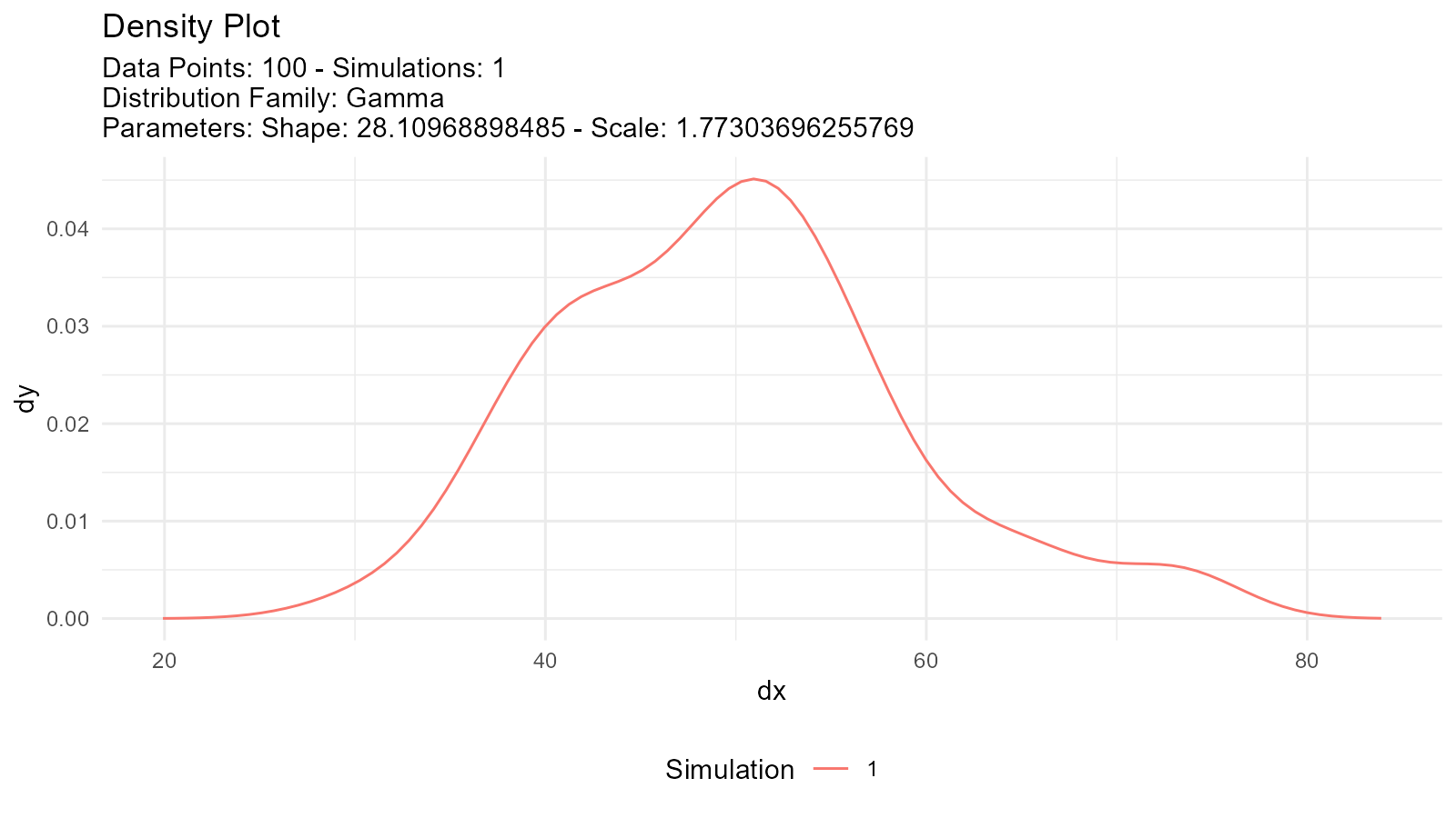

Advanced Techniques

1. Goodness-of-Fit Tests

Validate the fitted distribution:

# Fit distribution
data <- rnorm(100, mean = 50, sd = 10)
fit <- util_normal_param_estimate(data, .auto_gen_empirical = FALSE)

# Extract parameters
estimated_mean <- fit$parameter_tbl$mu[1]
estimated_sd <- fit$parameter_tbl$stan_dev[1]

# Kolmogorov-Smirnov test
ks.test(data, "pnorm", mean = estimated_mean, sd = estimated_sd)
#> 
#>  Asymptotic one-sample Kolmogorov-Smirnov test
#> 
#> data:  data
#> D = 0.041874, p-value = 0.9947
#> alternative hypothesis: two-sided

# Shapiro-Wilk test (for normality)
shapiro.test(data)
#> 
#>  Shapiro-Wilk normality test
#> 
#> data:  data
#> W = 0.99366, p-value = 0.9243

2. QQ Plot Validation

# Generate data for QQ plot
theoretical <- tidy_normal(
  .n = length(data),
  .mean = estimated_mean,
  .sd = estimated_sd
)

# Create QQ plot
tidy_autoplot(theoretical, .plot_type = "qq")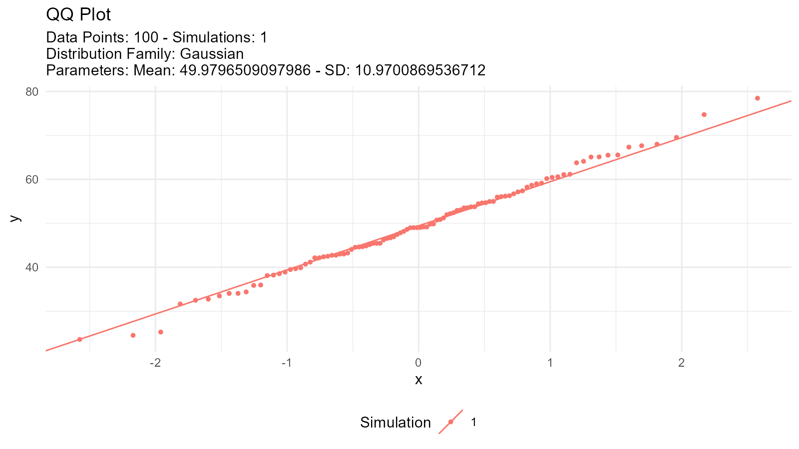

3. Residual Analysis

# Calculate residuals
# For a normal distribution, the expected value for each observation is the fitted mean
empirical <- tidy_empirical(.x = data, .num_sims = 1)
fitted <- tidy_normal(.n = length(data), .mean = estimated_mean, .sd = estimated_sd)
# Compare values
comparison <- data.frame(
  observed = data,
  expected = fitted$y[1:length(data)],
  residual = data - fitted$y[1:length(data)]
)
# Plot residuals
ggplot(comparison, aes(x = expected, y = residual)) +
  geom_point() +
  geom_hline(yintercept = 0, linetype = "dashed", color = "red") +
  labs(title = "Residual Plot", x = "Fitted Values", y = "Residuals")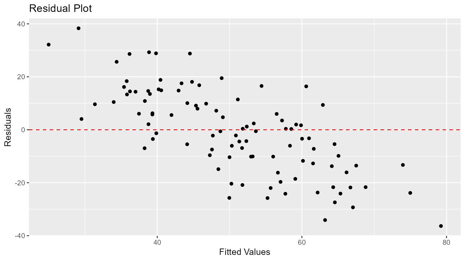

Statistics Tables

Distribution Statistics

Get summary statistics for fitted distributions:

# For normal distribution
util_normal_stats_tbl(tidy_normal()) |>
  glimpse()
#> Rows: 1
#> Columns: 17
#> $ tidy_function     <chr> "tidy_gaussian"
#> $ function_call     <chr> "Gaussian c(0, 1)"
#> $ distribution      <chr> "Gaussian"
#> $ distribution_type <chr> "continuous"
#> $ points            <dbl> 50
#> $ simulations       <dbl> 1
#> $ mean              <dbl> 0
#> $ median            <dbl> -0.08624274
#> $ mode              <dbl> 0
#> $ std_dv            <dbl> 1
#> $ coeff_var         <dbl> Inf
#> $ skewness          <dbl> 0
#> $ kurtosis          <dbl> 3
#> $ computed_std_skew <dbl> -0.09419539
#> $ computed_std_kurt <dbl> 2.993398
#> $ ci_lo             <dbl> -2.025975
#> $ ci_hi             <dbl> 1.917177

# For gamma distribution  
util_gamma_stats_tbl(tidy_gamma()) |>
  glimpse()
#> Rows: 1
#> Columns: 17
#> $ tidy_function     <chr> "tidy_gamma"
#> $ function_call     <chr> "Gamma c(1, 0.3)"
#> $ distribution      <chr> "Gamma"
#> $ distribution_type <chr> "continuous"
#> $ points            <dbl> 50
#> $ simulations       <dbl> 1
#> $ mean              <dbl> 1
#> $ mode              <dbl> 0
#> $ range             <chr> "0 to Inf"
#> $ std_dv            <dbl> 1
#> $ coeff_var         <dbl> 1
#> $ skewness          <dbl> 2
#> $ kurtosis          <dbl> 9
#> $ computed_std_skew <dbl> 0.9488492
#> $ computed_std_kurt <dbl> 3.56718
#> $ ci_lo             <dbl> 0.02308472
#> $ ci_hi             <dbl> 0.7102391

# For Poisson distribution
util_poisson_stats_tbl(tidy_poisson()) |>
  glimpse()
#> Rows: 1
#> Columns: 17
#> $ tidy_function     <chr> "tidy_poisson"
#> $ function_call     <chr> "Poisson c(1)"
#> $ distribution      <chr> "Poisson"
#> $ distribution_type <chr> "discrete"
#> $ points            <dbl> 50
#> $ simulations       <dbl> 1
#> $ mean              <dbl> 1
#> $ mode              <dbl> 1
#> $ range             <chr> "0 to Inf"
#> $ std_dv            <dbl> 1
#> $ coeff_var         <dbl> 1
#> $ skewness          <dbl> 1
#> $ kurtosis          <dbl> 4
#> $ computed_std_skew <dbl> 0.7359012
#> $ computed_std_kurt <dbl> 3.21436
#> $ ci_lo             <dbl> 0
#> $ ci_hi             <dbl> 3

Output includes:

• Mean
• Variance
• Standard deviation
• Skewness
• Kurtosis
• Mode (when applicable)
• Other distribution-specific statistics

Best Practices

1. Always Visualize

# Don't just look at parameters
fit <- util_normal_param_estimate(data, .auto_gen_empirical = TRUE)

# Always plot the comparison
fit$combined_data_tbl |>
  tidy_combined_autoplot()

2. Check Sample Size

n <- length(data)

if (n < 30) {
  message("Small sample size. Consider MVUE estimates.")
  message("Be cautious with MLE asymptotic properties.")
}

if (n < 10) {
  warning("Very small sample. Parameter estimates may be unreliable.")
}

3. Try Multiple Distributions

# Don't assume a distribution
# Try several and compare AIC

distributions <- c("normal", "lognormal", "gamma", "weibull")
aic_values <- numeric(length(distributions))

for (i in seq_along(distributions)) {
  aic_func <- get(paste0("util_", distributions[i], "_aic"))
  aic_values[i] <- aic_func(.x = data)
}

best_dist <- distributions[which.min(aic_values)]
message("Best fitting distribution: ", best_dist)

4. Validate Assumptions

# Check distributional assumptions

# 1. Visual check
fit <- util_normal_param_estimate(data, .auto_gen_empirical = TRUE)
fit$combined_data_tbl |>
  tidy_combined_autoplot()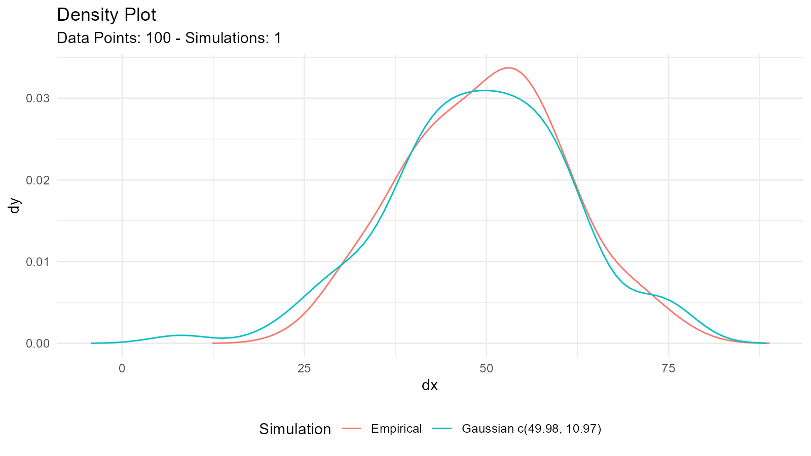

# 2. QQ plot
tidy_normal(.n = length(data), .mean = mean(data), .sd = sd(data)) |>
  tidy_autoplot(.plot_type = "qq")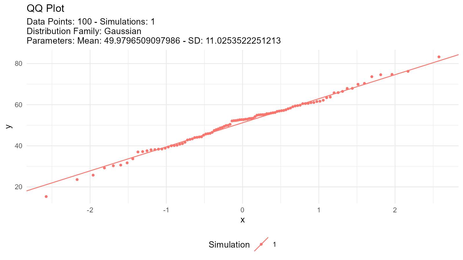

# 3. Statistical test
shapiro.test(data)  # For normality
#> 
#>  Shapiro-Wilk normality test
#> 
#> data:  data
#> W = 0.99366, p-value = 0.9243

5. Consider Data Characteristics

For positive continuous data:

• Try: Gamma, Weibull, Log-Normal, Exponential

For bounded data (0 to 1):

• Try: Beta distribution

For count data:

• Try: Poisson, Negative Binomial

For data with heavy tails:

• Try: Cauchy, Pareto, t-distribution

6. Document Your Process

# Good practice: Document your analysis

# Data source and characteristics
data <- mtcars$mpg
summary(data)
#>    Min. 1st Qu.  Median    Mean 3rd Qu.    Max. 
#>   10.40   15.43   19.20   20.09   22.80   33.90

# Try multiple distributions
normal_aic <- util_normal_aic(.x = data)
lognormal_aic <- util_lognormal_aic(.x = data)

# Select best fit
if (normal_aic < lognormal_aic) {
  best_fit <- util_normal_param_estimate(data, .auto_gen_empirical = TRUE)
  message("Normal distribution selected (AIC = ", round(normal_aic, 2), ")")
} else {
  best_fit <- util_lognormal_param_estimate(data, .auto_gen_empirical = TRUE)
  message("Log-normal distribution selected (AIC = ", round(lognormal_aic, 2), ")")
}

Common Issues and Solutions

Issue: Parameters Don’t Make Sense

Solution: Check your data for:

• Outliers
• Incorrect data type
• Missing values
• Inappropriate distribution choice

# Data diagnostics
summary(data)
#>    Min. 1st Qu.  Median    Mean 3rd Qu.    Max. 
#>   10.40   15.43   19.20   20.09   22.80   33.90
hist(data, main = "Histogram of Data", xlab = "Value")

boxplot(data, main = "Boxplot of Data", ylab = "Value")

Issue: Large Difference Between MLE and MVUE

Cause: Small sample size

Solution:

• Use MVUE for small samples
• Collect more data if possible
• Be cautious with interpretations

Issue: Poor Fit Quality

Solution:

• Try different distributions
• Check for mixture distributions
• Consider transforming data
• Look for outliers

Available Functions

Continuous Distributions

Distribution	Function
Normal	util_normal_param_estimate()
Log-Normal	util_lognormal_param_estimate()
Exponential	util_exponential_param_estimate()
Gamma	util_gamma_param_estimate()
Beta	util_beta_param_estimate()
Weibull	util_weibull_param_estimate()
Pareto	util_pareto_param_estimate()
Cauchy	util_cauchy_param_estimate()
Logistic	util_logistic_param_estimate()
Uniform	util_uniform_param_estimate()
Chi-Square	util_chisquare_param_estimate()
t-Distribution	util_t_param_estimate()

Discrete Distributions

Distribution	Function
Bernoulli	util_bernoulli_param_estimate()
Binomial	util_binomial_param_estimate()
Geometric	util_geometric_param_estimate()
Hypergeometric	util_hypergeometric_param_estimate()
Negative Binomial	util_negative_binomial_param_estimate()
Poisson	util_poisson_param_estimate()

Next Steps

• Bootstrap Analysis - Add robustness to your estimates
• Advanced Features - Mixture models and more
• Examples and Use Cases - Real-world applications

Ready for more advanced techniques? Continue to Bootstrap Analysis or Advanced Features vignettes!