Examples and Use Cases • TidyDensity

set.seed(123)
library(TidyDensity)
library(dplyr)
library(ggplot2)
library(patchwork)

Real-world examples demonstrating TidyDensity in action across various domains and applications.

Data Science and Analytics

Example 1: Exploring Customer Purchase Amounts

# Simulate customer purchase data
purchases <- c(rgamma(800, shape = 2, rate = 0.05),  # Regular customers
               rexp(200, rate = 0.01))                 # Big spenders

# Fit multiple distributions
normal_fit <- util_normal_param_estimate(purchases, .auto_gen_empirical = TRUE)
gamma_fit <- util_gamma_param_estimate(purchases, .auto_gen_empirical = TRUE)
lognormal_fit <- util_lognormal_param_estimate(purchases, .auto_gen_empirical = TRUE)

# Compare using AIC
aic_comparison <- data.frame(
  Distribution = c("Normal", "Gamma", "Log-Normal"),
  AIC = c(
    util_normal_aic(.x = purchases),
    util_gamma_aic(.x = purchases),
    util_lognormal_aic(.x = purchases)
  )
)

# Best distribution
best_dist <- aic_comparison[which.min(aic_comparison$AIC), ]
print(paste("Best fitting distribution:", best_dist$Distribution))
#> [1] "Best fitting distribution: Log-Normal"

# Visualize best fit
gamma_fit$combined_data_tbl |>
  tidy_combined_autoplot() +
  labs(title = "Customer Purchase Distribution",
       subtitle = paste("Best fit:", best_dist$Distribution),
       x = "Purchase Amount ($)",
       y = "Density")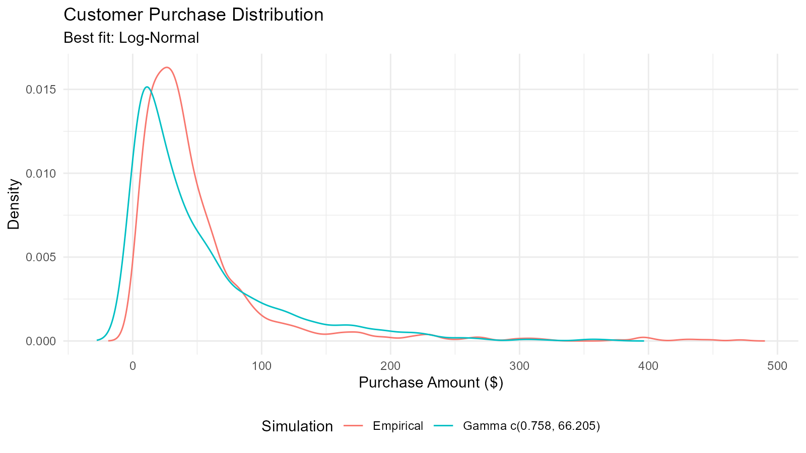

Density plot comparing the empirical distribution of simulated customer purchase data with a fitted gamma distribution, showing how TidyDensity can be used to identify the best-fitting distribution for business data

Example 2: A/B Test Analysis with Bootstrap

# Simulate A/B test data
group_a <- rnorm(100, mean = 50, sd = 10)  # Control
group_b <- rnorm(100, mean = 55, sd = 10)  # Treatment

# Bootstrap confidence intervals
bootstrap_diff <- function(n_sims = 5000) {
  diffs <- numeric(n_sims)
  for (i in 1:n_sims) {
    boot_a <- sample(group_a, length(group_a), replace = TRUE)
    boot_b <- sample(group_b, length(group_b), replace = TRUE)
    diffs[i] <- mean(boot_b) - mean(boot_a)
  }
  return(diffs)
}

# Run bootstrap
diff_distribution <- bootstrap_diff(5000)

# Calculate CI
ci <- quantile(diff_distribution, c(0.025, 0.975))
mean_diff <- mean(diff_distribution)

# Visualize
boot_tbl <- tidy_empirical(.x = diff_distribution, .num_sims = 1)
tidy_autoplot(boot_tbl, .plot_type = "density") +
  geom_vline(xintercept = ci[1], linetype = "dashed", color = "red") +
  geom_vline(xintercept = ci[2], linetype = "dashed", color = "red") +
  geom_vline(xintercept = 0, linetype = "solid", color = "black") +
  labs(title = "A/B Test: Difference in Means",
       subtitle = sprintf("95%% CI: [%.2f, %.2f]", ci[1], ci[2]),
       x = "Difference (B - A)",
       y = "Density")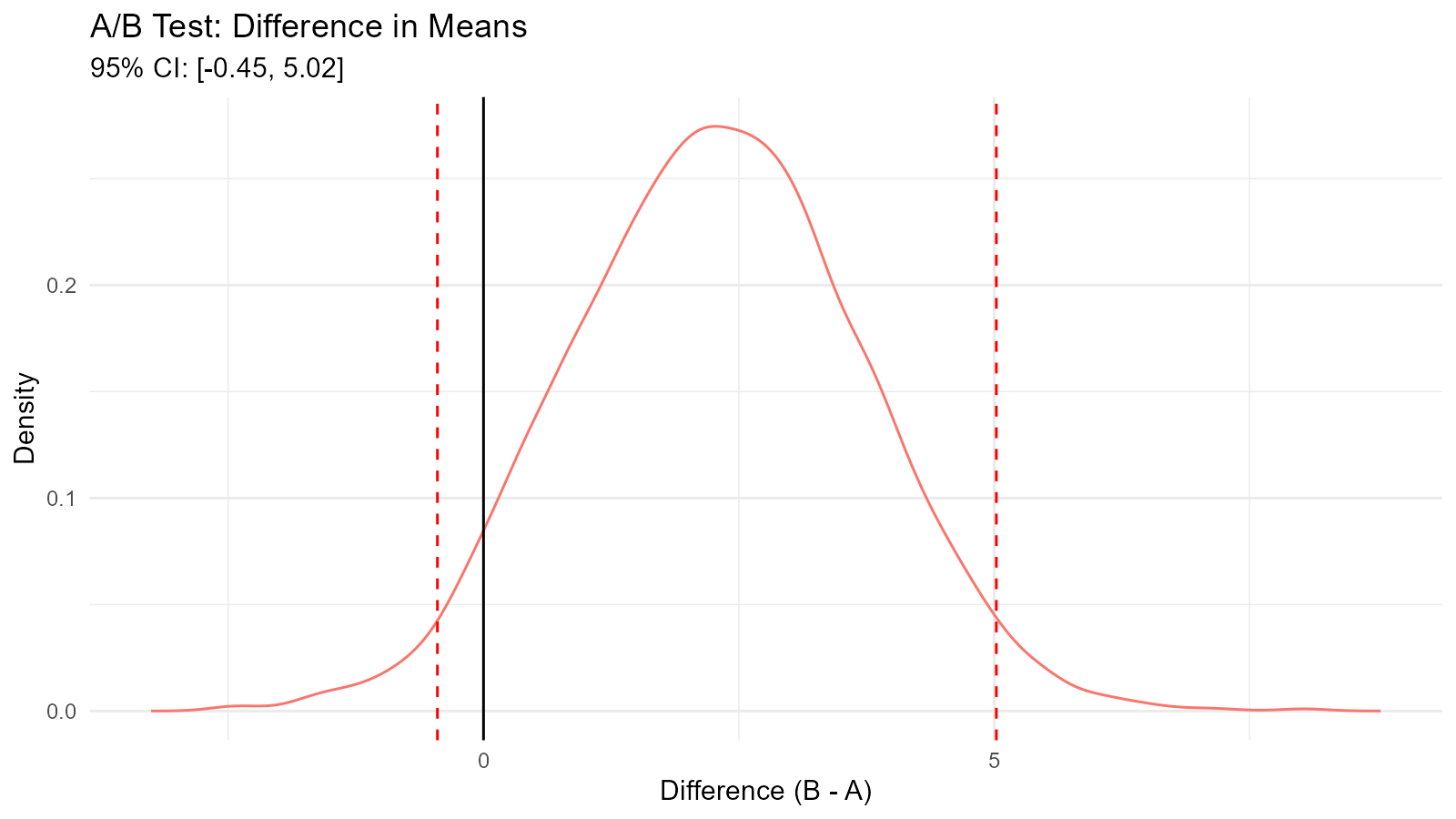

Density plot showing the bootstrap distribution of the difference in means between control and treatment groups in an A/B test, with vertical dashed lines indicating the 95% confidence interval bounds and a solid line at zero for reference


# Decision
if (ci[1] > 0) {
  cat("Result: Treatment B is significantly better (p < 0.05)\n")
} else if (ci[2] < 0) {
  cat("Result: Control A is significantly better (p < 0.05)\n")
} else {
  cat("Result: No significant difference detected\n")
}
#> Result: No significant difference detected

Example 3: Detecting Data Distribution Changes

# Before and after data
before <- rnorm(500, mean = 100, sd = 15)
after <- rnorm(500, mean = 105, sd = 20)  # Mean shift and more variance

# Generate distributions
dist_before <- tidy_empirical(.x = before, .num_sims = 1)
dist_after <- tidy_empirical(.x = after, .num_sims = 1)

# Combine for visualization
combined <- bind_rows(
  dist_before |> mutate(period = "Before"),
  dist_after |> mutate(period = "After")
)

# Plot
ggplot(combined, aes(x = y, fill = period)) +
  geom_density(alpha = 0.5) +
  labs(title = "Distribution Change Analysis",
       x = "Value",
       y = "Density",
       fill = "Period") +
  theme_minimal()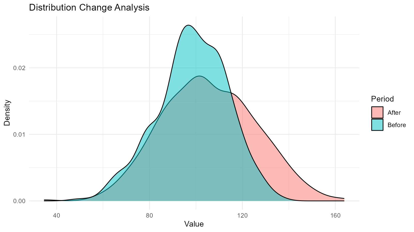

Overlaid density plots comparing 'Before' and 'After' distributions to detect changes in data characteristics such as mean shift and variance changes over time


# Statistical comparison
cat("Before: Mean =", round(mean(before), 2), ", SD =", round(sd(before), 2), "\n")
#> Before: Mean = 98.48 , SD = 15.2
cat("After:  Mean =", round(mean(after), 2), ", SD =", round(sd(after), 2), "\n")
#> After:  Mean = 105.61 , SD = 20.05

# Test for difference
t_test_result <- t.test(after, before)
cat("T-test p-value:", t_test_result$p.value, "\n")
#> T-test p-value: 3.793033e-10

Statistical Analysis

Example 4: Power Analysis for Sample Size Determination

# Simulate power analysis
effect_sizes <- seq(0.2, 1.0, by = 0.1)
sample_sizes <- seq(30, 200, by = 10)
power_results <- expand.grid(effect_size = effect_sizes, 
                             sample_size = sample_sizes)

# Calculate power for each combination
calculate_power <- function(n, effect) {
  simulations <- 1000
  significant <- 0
  
  for (i in 1:simulations) {
    group1 <- rnorm(n, mean = 0, sd = 1)
    group2 <- rnorm(n, mean = effect, sd = 1)
    p_value <- t.test(group1, group2)$p.value
    if (p_value < 0.05) significant <- significant + 1
  }
  
  return(significant / simulations)
}

# Run for a few key combinations (subset for speed)
key_combos <- power_results[c(1, 50, 100, 150), ] |> na.omit()
key_combos$power <- mapply(calculate_power, 
                           key_combos$sample_size,
                           key_combos$effect_size)

print(key_combos)
#>     effect_size sample_size power
#> 1           0.2          30 0.119
#> 50          0.6          80 0.968
#> 100         0.2         140 0.389
#> 150         0.7         190 1.000

Example 5: Distribution Goodness-of-Fit Testing

# Generate data (actually from gamma, but test multiple)
test_data <- rgamma(200, shape = 3, rate = 0.5)

# Fit multiple distributions and test
distributions <- list(
  "Normal" = function(x) util_normal_param_estimate(x, .auto_gen_empirical = FALSE),
  "Gamma" = function(x) util_gamma_param_estimate(x, .auto_gen_empirical = FALSE),
  "Weibull" = function(x) util_weibull_param_estimate(x, .auto_gen_empirical = FALSE),
  "Log-Normal" = function(x) util_lognormal_param_estimate(x, .auto_gen_empirical = FALSE)
)

# Calculate AIC for each
aic_results <- c(
  "Normal" = util_normal_aic(.x = test_data),
  "Gamma" = util_gamma_aic(.x = test_data),
  "Weibull" = util_weibull_aic(.x = test_data),
  "Log-Normal" = util_lognormal_aic(.x = test_data)
)

# Results
results_df <- data.frame(
  Distribution = names(aic_results),
  AIC = aic_results,
  Delta_AIC = aic_results - min(aic_results)
) |>
  arrange(AIC)

print(results_df)
#>            Distribution      AIC Delta_AIC
#> Gamma             Gamma 1009.000  0.000000
#> Log-Normal   Log-Normal 1013.549  4.549198
#> Weibull         Weibull 1023.253 14.253167
#> Normal           Normal 1082.418 73.417824
cat("\nBest fitting distribution:", results_df$Distribution[1], "\n")
#> 
#> Best fitting distribution: Gamma

Finance and Risk Management

Example 6: Value at Risk (VaR) Calculation

# Simulate daily returns
returns <- rnorm(1000, mean = 0.001, sd = 0.02)  # 0.1% daily return, 2% volatility

# Create distribution
returns_dist <- tidy_empirical(.x = returns, .num_sims = 1)

# Calculate VaR at different confidence levels
var_95 <- quantile(returns, 0.05)
var_99 <- quantile(returns, 0.01)
var_995 <- quantile(returns, 0.005)

# Bootstrap for VaR confidence intervals
boot_returns <- tidy_bootstrap(.x = returns, .num_sims = 2000)

boot_var <- boot_returns |>
  bootstrap_unnest_tbl() |>
  group_by(sim_number) |>
  summarise(var_95 = quantile(y, 0.05)) |>
  ungroup()

var_ci <- quantile(boot_var$var_95, c(0.025, 0.975))

# Results
cat("Value at Risk (VaR) Analysis\n")
#> Value at Risk (VaR) Analysis
cat("95% VaR:", round(var_95 * 100, 3), "%\n")
#> 95% VaR: -3.199 %
cat("99% VaR:", round(var_99 * 100, 3), "%\n")
#> 99% VaR: -4.479 %
cat("99.5% VaR:", round(var_995 * 100, 3), "%\n")
#> 99.5% VaR: -5.064 %
cat("\n95% CI for 95% VaR: [", round(var_ci[1] * 100, 3), "%,", 
    round(var_ci[2] * 100, 3), "%]\n")
#> 
#> 95% CI for 95% VaR: [ -3.386 %, -2.958 %]

# Visualize
tidy_autoplot(returns_dist, .plot_type = "density") +
  geom_vline(xintercept = var_95, color = "orange", linetype = "dashed") +
  geom_vline(xintercept = var_99, color = "red", linetype = "dashed") +
  annotate("text", x = var_95, y = 0, label = "95% VaR", vjust = -1) +
  annotate("text", x = var_99, y = 0, label = "99% VaR", vjust = -1) +
  labs(title = "Portfolio Returns Distribution with VaR",
       x = "Daily Return",
       y = "Density")

Density plot of simulated daily portfolio returns showing the distribution with vertical dashed lines marking the 95% and 99% Value at Risk thresholds, used for risk management analysis

Example 7: Option Pricing with Monte Carlo Simulation

# Simulate stock price paths using GBM
stock_price_simulation <- function(S0, mu, sigma, T, n_steps, n_sims) {
  dt <- T / n_steps
  paths <- matrix(0, nrow = n_steps + 1, ncol = n_sims)
  paths[1, ] <- S0
  
  for (i in 2:(n_steps + 1)) {
    Z <- rnorm(n_sims)
    paths[i, ] <- paths[i-1, ] * exp((mu - 0.5 * sigma^2) * dt + sigma * sqrt(dt) * Z)
  }
  
  return(paths)
}

# Parameters
S0 <- 100      # Initial stock price
K <- 105       # Strike price
mu <- 0.05     # Drift
sigma <- 0.2   # Volatility
T <- 1         # Time to maturity (1 year)
n_steps <- 252 # Daily steps
n_sims <- 1000

# Simulate
paths <- stock_price_simulation(S0, mu, sigma, T, n_steps, n_sims)

# Final prices
final_prices <- paths[nrow(paths), ]

# Option payoffs
call_payoffs <- pmax(final_prices - K, 0)
put_payoffs <- pmax(K - final_prices, 0)

# Expected values (discounted)
r <- 0.03  # Risk-free rate
call_price <- mean(call_payoffs) * exp(-r * T)
put_price <- mean(put_payoffs) * exp(-r * T)

cat("Call Option Price:", round(call_price, 2), "\n")
#> Call Option Price: 8.12
cat("Put Option Price:", round(put_price, 2), "\n")
#> Put Option Price: 7.74

# Visualize final price distribution
final_dist <- tidy_empirical(.x = final_prices, .num_sims = 1)
tidy_autoplot(final_dist, .plot_type = "density") +
  geom_vline(xintercept = K, color = "red", linetype = "dashed") +
  geom_vline(xintercept = S0, color = "blue", linetype = "dashed") +
  labs(title = "Simulated Stock Price Distribution at Maturity",
       x = "Stock Price",
       y = "Density")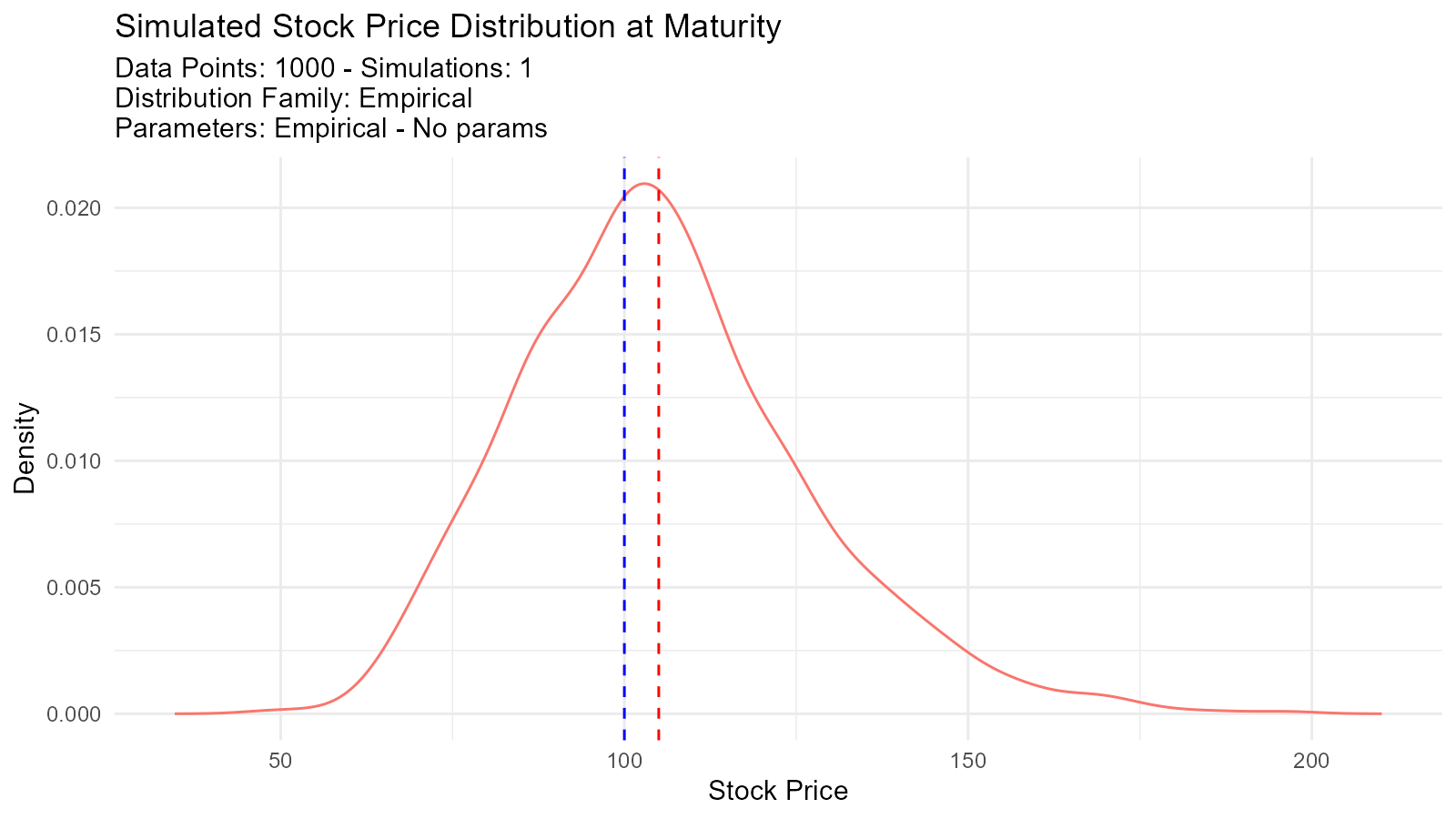

Density plot showing the simulated distribution of stock prices at option maturity using geometric Brownian motion, with vertical lines indicating the current stock price and strike price for option pricing analysis

Quality Control and Manufacturing

Example 8: Process Capability Analysis

# Manufacturing process data
measurements <- rnorm(500, mean = 100, sd = 2)  # Target = 100
LSL <- 94  # Lower specification limit
USL <- 106 # Upper specification limit

# Fit distribution
fit <- util_normal_param_estimate(measurements, .auto_gen_empirical = TRUE)
mean_est <- fit$parameter_tbl$mu[1]
sd_est <- fit$parameter_tbl$stan_dev[1]

# Calculate Cp and Cpk
Cp <- (USL - LSL) / (6 * sd_est)
Cpu <- (USL - mean_est) / (3 * sd_est)
Cpl <- (mean_est - LSL) / (3 * sd_est)
Cpk <- min(Cpu, Cpl)

# Defect rate
defect_rate <- (pnorm(LSL, mean_est, sd_est) + 
                (1 - pnorm(USL, mean_est, sd_est))) * 100

# Results
cat("Process Capability Analysis\n")
#> Process Capability Analysis
cat("Cp:", round(Cp, 3), "\n")
#> Cp: 0.988
cat("Cpk:", round(Cpk, 3), "\n")
#> Cpk: 0.971
cat("Estimated Defect Rate:", round(defect_rate, 4), "%\n")
#> Estimated Defect Rate: 0.307 %

# Interpretation
if (Cpk >= 1.33) {
  cat("Process capability: GOOD\n")
} else if (Cpk >= 1.0) {
  cat("Process capability: ADEQUATE\n")
} else {
  cat("Process capability: POOR - Action required\n")
}
#> Process capability: POOR - Action required

# Visualize
fit$combined_data_tbl |>
  tidy_combined_autoplot() +
  geom_vline(xintercept = LSL, color = "red", linetype = "dashed") +
  geom_vline(xintercept = USL, color = "red", linetype = "dashed") +
  geom_vline(xintercept = 100, color = "blue", linetype = "solid") +
  labs(title = "Process Capability Analysis",
       subtitle = sprintf("Cp = %.3f, Cpk = %.3f", Cp, Cpk),
       x = "Measurement",
       y = "Density")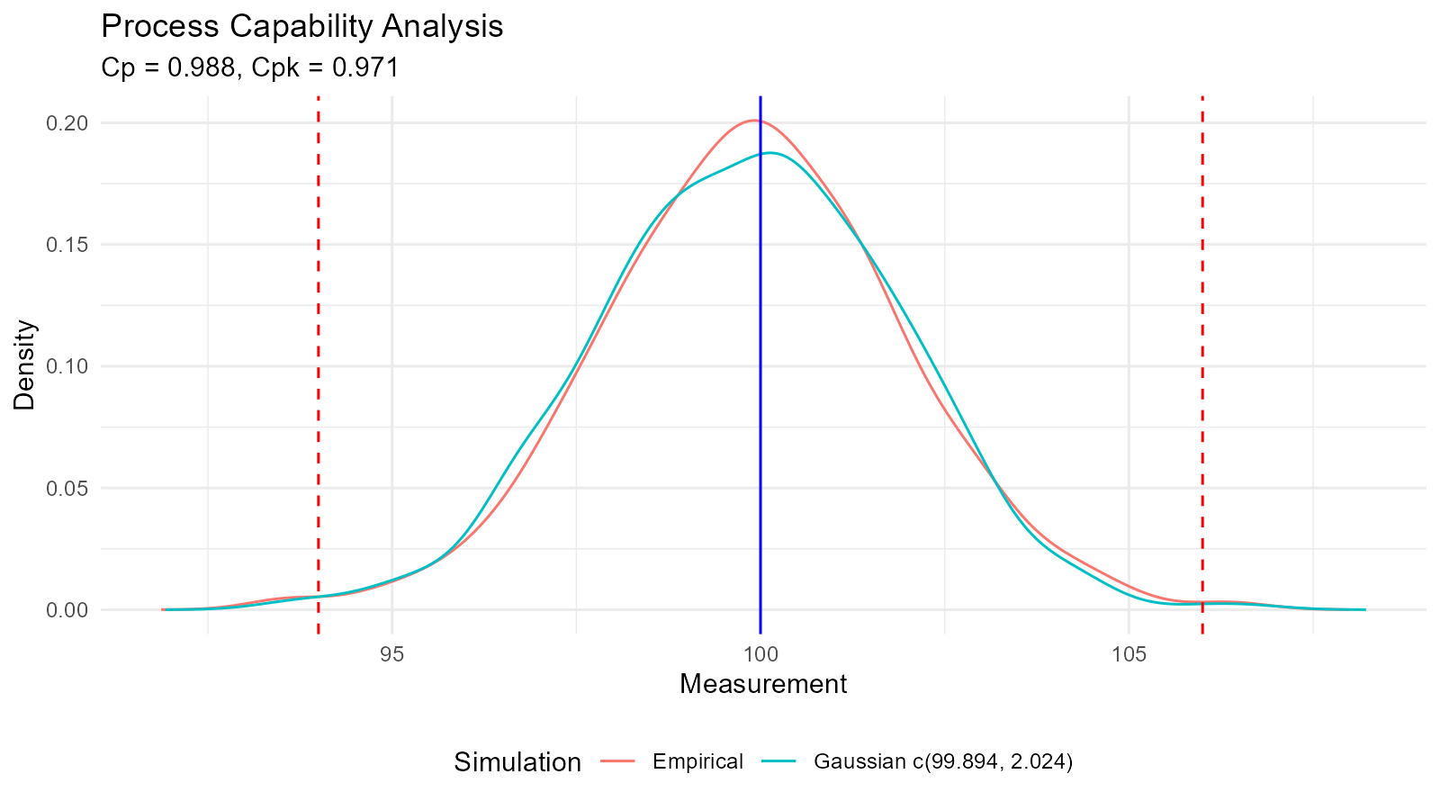

Density plot showing the distribution of manufacturing measurements overlaid with specification limits (LSL and USL) and target value, with process capability indices Cp and Cpk displayed in the subtitle

Example 9: Control Chart Analysis

# Generate process data with a shift
n_before <- 200
n_after <- 50
before_shift <- rnorm(n_before, mean = 100, sd = 3)
after_shift <- rnorm(n_after, mean = 105, sd = 3)  # Process shifted

all_data <- c(before_shift, after_shift)
time <- 1:length(all_data)

# Calculate control limits
mean_val <- mean(before_shift)
sd_val <- sd(before_shift)
UCL <- mean_val + 3 * sd_val
LCL <- mean_val - 3 * sd_val

# Create control chart
control_data <- data.frame(time = time, value = all_data)

ggplot(control_data, aes(x = time, y = value)) +
  geom_line() +
  geom_point() +
  geom_hline(yintercept = mean_val, color = "blue") +
  geom_hline(yintercept = UCL, color = "red", linetype = "dashed") +
  geom_hline(yintercept = LCL, color = "red", linetype = "dashed") +
  geom_vline(xintercept = n_before, color = "orange", linetype = "dotted") +
  labs(title = "X-bar Control Chart",
       subtitle = "Process Shift Detected",
       x = "Sample",
       y = "Measurement") +
  theme_minimal()

X-bar control chart showing process measurements over time with horizontal lines for the mean and upper/lower control limits (UCL/LCL), and a vertical line indicating where a process shift occurred

Healthcare and Epidemiology

Example 10: Disease Outbreak Modeling

# Model daily case counts with Poisson distribution
days <- 1:90
baseline_rate <- 5
peak_rate <- 50

# Simulate outbreak with time-varying rate
lambda <- baseline_rate + (peak_rate - baseline_rate) * 
  exp(-((days - 45)^2) / (2 * 15^2))  # Gaussian curve

cases <- rpois(length(days), lambda)

# Fit Poisson distribution to peak period
peak_cases <- cases[35:55]
poisson_fit <- util_poisson_param_estimate(peak_cases, .auto_gen_empirical = TRUE)

# Visualize time series
outbreak_data <- data.frame(day = days, cases = cases, expected = lambda)

p1 <- ggplot(outbreak_data, aes(x = day, y = cases)) +
  geom_point() +
  geom_line(aes(y = expected), color = "red", linetype = "dashed") +
  labs(title = "Disease Outbreak Time Series",
       subtitle = "Observed Cases vs Expected Rate",
       x = "Day",
       y = "Number of Cases") +
  theme_minimal()

# Peak analysis
p2 <- poisson_fit$combined_data_tbl |>
  tidy_combined_autoplot() +
  labs(title = "Peak Period Case Distribution",
       x = "Daily Cases",
       y = "Density")

p1 / p2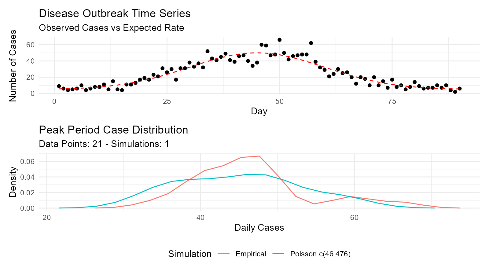

Two-panel display showing (1) a time series of daily disease cases with observed counts as points and the expected rate as a red dashed line, and (2) a density plot of the case distribution during the peak outbreak period fitted with a Poisson distribution

Machine Learning and Simulation

Example 11: Monte Carlo Simulation for Project Planning

# Project task duration simulation using triangular distribution
tasks <- list(
  task1 = list(min = 5, mode = 8, max = 15),
  task2 = list(min = 3, mode = 5, max = 10),
  task3 = list(min = 7, mode = 10, max = 20),
  task4 = list(min = 2, mode = 4, max = 8)
)

# Simulate total project duration
n_sims <- 5000
total_durations <- numeric(n_sims)

for (i in 1:n_sims) {
  task_durations <- sapply(tasks, function(task) {
    tidy_triangular(.n = 2, .min = task$min, .max = task$max, .mode = task$mode)$y[1]
  })
  total_durations[i] <- sum(task_durations)
}

# Analyze results
duration_dist <- tidy_empirical(.x = total_durations, .num_sims = 1)

percentiles <- quantile(total_durations, c(0.1, 0.5, 0.9))

cat("Project Duration Analysis\n")
#> Project Duration Analysis
cat("10th percentile (optimistic):", round(percentiles[1], 1), "days\n")
#> 10th percentile (optimistic): 27.2 days
cat("50th percentile (median):", round(percentiles[2], 1), "days\n")
#> 50th percentile (median): 32.3 days
cat("90th percentile (pessimistic):", round(percentiles[3], 1), "days\n")
#> 90th percentile (pessimistic): 37.7 days

# Visualize
tidy_autoplot(duration_dist, .plot_type = "density") +
  geom_vline(xintercept = percentiles[1], color = "green", linetype = "dashed") +
  geom_vline(xintercept = percentiles[2], color = "blue", linetype = "solid") +
  geom_vline(xintercept = percentiles[3], color = "red", linetype = "dashed") +
  labs(title = "Project Duration Distribution",
       subtitle = "Monte Carlo Simulation (5000 iterations)",
       x = "Total Duration (days)",
       y = "Density")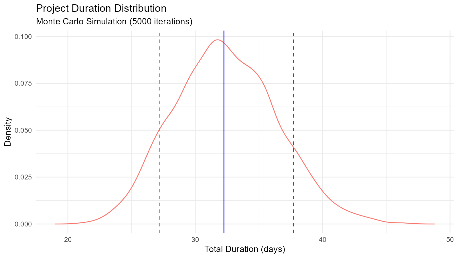

Density plot showing the Monte Carlo simulated distribution of total project duration with vertical lines marking the 10th percentile (optimistic), 50th percentile (median), and 90th percentile (pessimistic) estimates

Education and Teaching

Example 12: Demonstrating Central Limit Theorem

# Show CLT with different source distributions
n_samples <- 1000
sample_sizes <- c(5, 10, 30, 50)

demonstrate_clt <- function(source_dist_func, sample_size, n_samples) {
  sample_means <- numeric(n_samples)
  for (i in 1:n_samples) {
    sample <- source_dist_func(sample_size)
    sample_means[i] <- mean(sample)
  }
  return(sample_means)
}

# Source: Uniform distribution
uniform_source <- function(n) runif(n, 0, 1)

# Generate for different sample sizes
results <- lapply(sample_sizes, function(n) {
  means <- demonstrate_clt(uniform_source, n, n_samples)
  tidy_empirical(.x = means, .num_sims = 1) |>
    mutate(sample_size = n)
})

# Combine and plot
combined <- bind_rows(results)

ggplot(combined, aes(x = y)) +
  geom_density(fill = "skyblue", alpha = 0.5) +
  facet_wrap(~sample_size, scales = "free", 
             labeller = labeller(sample_size = function(x) paste("n =", x))) +
  labs(title = "Central Limit Theorem Demonstration",
       subtitle = "Sample Means from Uniform(0,1) Distribution",
       x = "Sample Mean",
       y = "Density") +
  theme_minimal()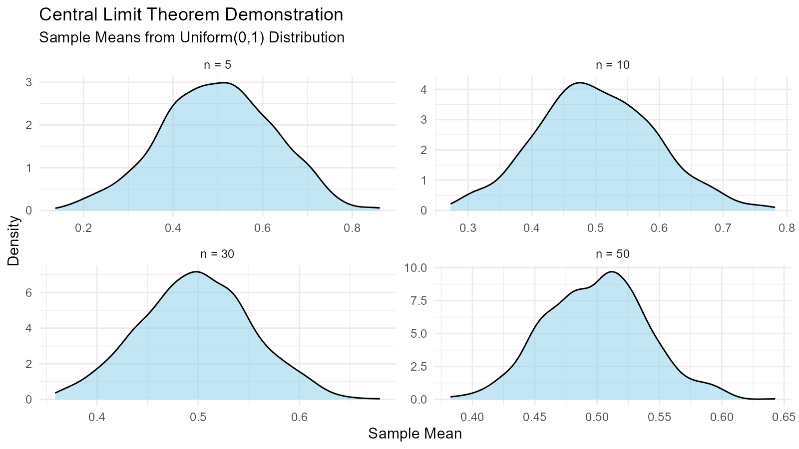

Four-panel density plot showing how the distribution of sample means from a uniform distribution becomes more normal as sample size increases from n=5 to n=50, demonstrating the Central Limit Theorem

Tips for Your Own Use Cases

1. Start with Exploration

# Explore your data
summary(your_data)
hist(your_data)

# Try empirical distribution
emp <- tidy_empirical(.x = your_data, .num_sims = 1)
tidy_autoplot(emp, .plot_type = "density")

2. Try Multiple Distributions

# Systematic comparison
distributions <- c("normal", "gamma", "lognormal", "weibull")
aics <- sapply(distributions, function(d) {
  func <- get(paste0("util_", d, "_aic"))
  func(.x = your_data)
})
best <- distributions[which.min(aics)]

3. Validate with Visualization

# Always visualize
fit <- get(paste0("util_", best, "_param_estimate"))(
  your_data,
  .auto_gen_empirical = TRUE
)

fit$combined_data_tbl |>
  tidy_combined_autoplot()

4. Use Bootstrap for Uncertainty

# Add bootstrap confidence intervals
boot <- tidy_bootstrap(.x = your_data, .num_sims = 2000)
boot |>
  bootstrap_unnest_tbl() |>
  summarise(
    lower = quantile(y, 0.025),
    upper = quantile(y, 0.975)
  )

Key Takeaways

1. Distribution Fitting is Essential

Use AIC to compare multiple candidate distributions and select the best fit for your data.

2. Bootstrap Provides Robust Uncertainty

When parametric assumptions are uncertain, bootstrap resampling gives reliable confidence intervals.

3. Visualization Validates Analysis

Always plot your results to verify that fitted distributions match the empirical data.

4. TidyDensity Integrates with Tidyverse

Leverage dplyr, ggplot2, and other tidyverse tools for seamless analysis workflows.

5. Domain Knowledge Guides Choices

Let your understanding of the problem domain inform distribution selection and interpretation.